Steps In Quantitative Data Analysis 5k4v64

1 Steps in Quantitative Data Analysis 1.

Preparing the data – before a researcher can analyze his data through quantitative data analysis, he/she must first change every data in numerical information or to quantify the data.

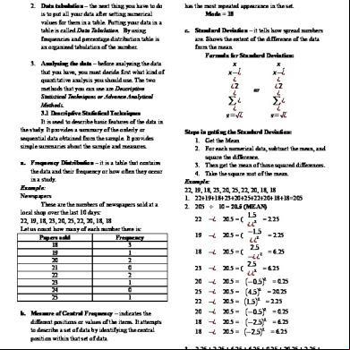
2. Data tabulation – the next thing you have to do is to put all your data after setting numerical values for them in a table. Putting your data in a table is called Data Tabulation. By using frequencies and percentage distribution table is an organized tabulation of the number. 3. Analyzing the data – before analyzing the data that you have, you must decide first what kind of quantitative analysis you should use. The two methods that you can use are Descriptive Statistical Techniques or Advance Analytical Methods. 3.1 Descriptive Statistical Techniques It is used to describe basic features of the data in the study. It provides a summary of the orderly or sequential data obtained from the sample. It provides simple summaries about the sample and measures. a. Frequency Distribution – it is a table that contains the data and their frequency or how often they occur in a study. Example: Newspapers These are the numbers of newspapers sold at a local shop over the last 10 days: 22, 19, 18, 23, 20, 25, 22, 20, 18, 18 Let us count how many of each number there is: Papers sold Frequency 18 3 19 1 20 2 21 0 22 2 23 1 24 0 25 1

b.2.Median – the score in the middle of the set of items that cuts or divides the set into two groups. Example: 22, 19, 18, 23, 20, 25, 22, 20, 18, 18 18, 18, 18, 19, 20, 20, 22, 22, 23, 25 Median = 20 b.3. Mode refers to the item or score in the data set that has the most repeated appearance in the set. Mode = 18 c. Standard Deviation – it tells how spread numbers are. Shows the extent of the difference of the data from the mean. Formula for Standard Deviation:

x x−¿´ ¿ ¿2 ¿ ∑¿ ¿ s= √ ¿

Steps in getting the Standard Deviation: 1. Get the Mean 2. For each numerical data, subtract the mean, and square the difference. 3. Then get the mean of those squared differences. 4. Take the square root of the mean. Example: 22, 19, 18, 23, 20, 25, 22, 20, 18, 18 1. 22+19+18+23+20+25+22+20+18+18=205 2. 205 ÷ 10 = 20.5 (MEAN) 22

−¿

19

−¿

18

−¿

23

−¿

20

−¿ −¿ −¿ −¿ −¿ −¿

25 22 20

b. Mesaure of Central Frequency – indicates the different positions or values of the items. It attempts to describe a set of data by identifying the central position within that set of data. b.1. Mean – average of all the items or scores. It can be denoted by a variable with a line on top (e.g. X´ , Y´ ). Example: 22, 19, 18, 23, 20, 25, 22, 20, 18, 18 22+19+18+23+20+25+22+20+18+18=205 205 ÷ 10= 20.5 (MEAN)

or

x x−¿´ ¿ ¿2 ¿ ∑¿ ¿ s= √ ¿

18 18

1.5 = 2.25 ¿ ¿2 −1.5 20.5 = ( = 2.25 ¿ ¿2 2.5 20.5 = ( = 6.25 −¿ ¿ 2 2.5 20.5 = ( = 6.25 ¿ ¿2 20.5 = (−0.5)2 = 0.25 20.5 = (4.5)2 = 20.25 20.5 = (1.5)2 = 2.25 20.5 = (−0.5)2 = 0.25 20.5 = (−2.5)2 = 6.25 20.5 = (−2.5)2 = 6.25 20.5 = (

3. 2.25 + 2.25 + 6.25 + 6.25 + 0.25 + 20.25 + 2.25 + 0.25 + 6.25 + 6.25= 52.5 MEAN = 5.83 4.

√ 5.83

= 2.41, Standard Deviation = 2.41

2

x x−¿´ ¿ ¿2 *NOTE: we use if the mean is given, ¿ ∑¿ ¿ s= √ ¿ x x−¿´ ¿ ¿2 while we use ¿ ∑¿ ¿ s= √ ¿

if we calculate the mean

ourselves. d. Variance – It is the square of the Standard Deviation. Example: 22, 19, 18, 23, 20, 25, 22, 20, 18, 18 Standard Deviation = 2.41 Variance = 5.81

e. Covariance Formula:

¿

¿

∑ ( X− X´ ) (Y −Y´ ) n

∑ ( X− X´ ) (Y −Y´ ) n−1

Example: Student 1 2 3 4 5

or

, we let sample = n

Scores (X) 30 25 15 26 18

Study Hours (Y) 4 3 1 4 2

To compute the covariance: ´ )( - First we have to get the summation of “( X − X Y −Y´ ¿ ”

∑ “( X− X´ )(Y −Y´ )

= 30.44 - Then we must divide it to the number of sample - 1 - So 30.44/5 = 6.09 - So the COVARIANCE = 6.09 - So our formula for the COVARIANCE is

¿

∑ ( X− X´ ) (Y −Y´ ) n

Example: We will try to determine the correlation between study hours and exam scores. Student Scores Study Hours 1 30 4 2 25 3 3 15 1 4 26 4 5 18 2 First thing to do is to find the variance of the “scores”: Let X be the Scores” ( ( Student X X´ ´

X −X ¿

covariance √ variance 1 x variance 2

=

6.09 √28.49 x 1.36

= 0.98

3.2 Advance Quantitative Analytical Methods.

X −¿´2 ¿

1 30 7.2 51.84 2 25 2.5 6.25 3 15 -7.5 51.84 4 26 3.5 12.25 5 18 -4.5 20.25 MEAN = 22.8 STANDARD DEVIATION = 5.34 VARIANCE = 28.49 Then get the VARIANCE of the “study hours”: Let Y be Study Hours ( Studnet

Y

( Y −Y´ ¿

Y´ Y −¿´2 ¿

1 4 1.2 2 3 0.2 3 1 -1.8 4 4 1.2 5 2 -0.8 MEAN = 2.8 STANDARD DEVIATION = 1.17 VARIANCE = 1.36 Now let us compute for the covariance Let x = (Socres – Mean) Y = (Study hours – Mean)

, we let sample = n

Finally to get the correlation (r), Let r be the correlation

r=

Is an analysis of quantitative data that involves the use of a more complex statistical method. a. Correlation – uses statistical analysis to gain results that that can describe the relationship between two variables. It cannot, however, establich causal relationship. We need to use Variance and Covariance to solve the Correlation.

( Students

X − X´´

1 2 3 4 5

) 7.2 2.5 -7.5 3.5 -4.5

( Y −Y´´ ) 1.2 0.2 -1.8 1.2 -0.8

1.44 0.04 3.24 1.44 0.64

´´ )( ( X −X

Y −Y´´ ) 8.64 0.5 13.5 4.2 3.6

3

( X −¿ X )(Y −Y ) ∑¿ =30.44 To compute the covariance: ´ )( - First we have to get the summation of “( X − X Y −Y´ ¿ ”

∑ “( X− X´ )(Y −Y´ )

= 30.44 - Then we must divide it to the number of sample - 1 - So 30.44/5 = 6.09 - So the COVARIANCE = 6.09 - So our formula for the COVARIANCE is

¿

∑ ( X− X´ ) (Y −Y´ ) n

, we let sample = n

Finally to get the correlation (r), Let r be the correlation

r=

covariance √ variance 1 x variance 2

=

6.09 √28.49 x 1.36

= 0.98 As we noted, sample correlation coefficients may range from -1 to +1. In practice, meaningful correlations can be as small as 0.4 to -0.4 for positive or negative associations.