Asme Guide For Verification And Validation Of Mechnics Software 602112

Reprinted by permission of The American Society of Mechanical Engineers. All rights reserved.

An Overview of the PTC 60 / V&V 10

Guide for Verification and Validation in Computational Solid Mechanics Transmitted by L.E. Schwer, Chair PTC 60 /V&V 10

Preface The American Society of Mechanical Engineers (ASME) Standards Committee on Verification and Validation in Computational Solid Mechanics (PTC 60/V&V 10) approved their first document (Guide) in July 2006. The Guide has been submitted to ASME publications and to the American National Standards Institute (ANSI) for public review. It is hoped the Guide will be published in early 2007.

Some Motivation Question: Are the sometimes lengthy and costly processes of verification & validation really necessary? Consider the following scenario that perhaps you can relate to first hand. A project review meeting is taking place and the project manager needs to make a critical decision to accept or reject a proposed design change. A relatively new employee, freshly minted from the nearby engineering university, makes an impressive presentation full of colorful slides of deformed meshes and skillfully crafted line plots indicating the results of many U and labor hours of non-linear numerical analyses, ending with a recommendation to accept the design change. Hopefully, an astute project manager, aware of the vagaries of nonlinear numerical analyses, will not accept the analysis and its conclusion at face value, especially given the inexperience of the analyst. Rather, the project manager should seek some assurance that not only are the results reasonable, but a sound procedure was followed in developing the model and documenting the numerous physical and numerical parameters required for a typical analysis. The degree of assurance sought by the project manager is directly related to the criticality of the decision to be made.

1

Reprinted by permission of The American Society of Mechanical Engineers. All rights reserved.

The processes of verification & validation are how evidence is collected, and documented, that help establish confidence in the results of complex numerical simulations.

A Brief History of the Committee In 1999 an ad hoc verification & validation specialty committee was formed under the auspices of the United States Association for Computational Mechanics (USACM). The purpose of this committee was to pursue the formation of a verification & validation standards committee under a professional engineering society approved to produce standards under the rules of the American National Standards Institute (ANSI). This goal was achieved in 2001 when the then Board on Performance Test Codes (PTC) of the American Society of Mechanical Engineers (ASME) approved the committee’s charter: To develop standards for assessing the correctness and credibility of modeling and simulation in computational solid mechanics. and the committee was assigned the title and designation of the ASME Committee for Verification & Validation in Computational Solid Mechanics (PTC 601). The committee maintains a roster of slightly less than the maximum permitted 30 , with a few alternate and corresponding . The hip is diverse with three major groups being industry, Government, and academia. The industry include representatives from auto and aerospace industries and the Government are primarily from the Departments of Defense and Energy. Particularly well represented are from the three national laboratories under the National Nuclear Security istration. This latter hip group is key to the committee as much of the recent progress in verification & validation has come from these laboratories and their efforts under the Advanced Simulation and Computing (ASC) Program, started in 1995.

A Brief History of the Guide The motivation for forming the ASME committee was provided by PTC 60’s elder ‘sister’ committee, the Computational Fluid Dynamics Committee of the American Institute of Aeronautics and Astronautics (AIAA). After the 1998 publication of their seminal work in verification & validation, i.e. the AIAA Guide for the Verification and Validation of Computational Fluid Dynamics Committee on Standards, the AIAA CFD committee thought it would be good for the overall computational mechanics community, if the solid and structural2 mechanics community produced a similar guide.

1 2

The committee may be designated as V&V 10 in the near future. Hereafter referred to as “solid mechanics” for brevity.

2

Reprinted by permission of The American Society of Mechanical Engineers. All rights reserved.

The road from committee formation to approval of the Guide was neither straight nor fast, but it was rewarding. Starting from the naive idea that the AIAA Guide could easily be modified to suit the purposes of computational solid mechanics, the committee soon realized that forming a consensus means understanding the point of view of others, and it is the significant effort expended in forming of a consensus view that lends authority to standards documents such as the present Guide. While some may view five years to produce a 30+ page Guide as an excessive amount of time, several factors contributed to this duration: 1. PTC 60 was a newly formed committee, and thus time was need for the group to become cohesive, 2. This is an all volunteer committee with the donating most generously of their time and resources, 3. The area of verification & validation is growing rapidly, with improvements arriving at a pace that caused the committee to revisit the initial parts of the Guide and include important improvements in V&V. After an extensive Industry Review process, and associated changes to Guide, the committee unanimously approved the Guide in a ballot concluded on 13 July 2006. The Guide has successfully completed its public review under ASME standard procedures and been approved by the American National Standards Institute (ANSI). The Guide is presently in ASME publications and has been given high priority for publication. It is hoped the Guide will be published in December 2006, or early 2007.

What the Guide is Not Perhaps the most common misconception about the Guide is that it would provide a definitive step-by-step V&V procedure, immediately applicable by analysts in computational mechanics. This expectation is quite understandable when viewed by an outsider to the V&V community. One reads a title page with words ASME standards committee and verification & validation, and expects a typical ASME standards document. Somehow the reader glosses over the very intentional first word of the title, i.e. Guide - something that offers underlying information. Not only the first time reader, but much of the informed V&V computational mechanics community desires a step-by-step standard. However, it is the view of the committee that such a standard is many years in the future. The next immediate goal for PTC 60, and its AIAA Computational Fluid Dynamics Standards sister committee, is to attempt to define some best practices, which in the future can lead to standards; our ASME sister committee, PTC 61/V&V 20, is already addressing best practices for uncertainty analysis related to some aspects of V&V. The committee makes no excuses for writing the present Guide the way it did. After five years of discussion and debate, the committee recognizes it was a necessary, but difficult, first step. Much of V&V is not a ‘hard’ science, which is the bread-and-butter of most of computational mechanics, but more a ‘soft’ science like the philosophy of science, where differing points of view have merit, and need not be evaluated as either right or wrong.

3

Reprinted by permission of The American Society of Mechanical Engineers. All rights reserved.

Because the present Guide is intentionally a foundational document, and not a typical ASME standard, the committee deviated significantly from the well-developed guidance for writing standards documents, provided by both the ASME Codes & Standards Council and the PTC Committee. Attempting to force this Guide into an ASME standard format would detract significantly from its appeal to potential readers. The intended audience for this Guide is not the occasional computational mechanics , e.g. a modern-day draftsman using an automated CAD/FEA package, rather it is computational analysts, experimentalists, code developers, and physics model developers, and their managers, who are prepared to read a technical document with a mixture of discussion concerning mathematics, numerics, experimentation, and engineering analysis processes.

Outline of the Guide As stated in the Guide’s Abstract, the guidelines are based on the following key principles: • • • • •

Verification must precede validation. The need for validation experiments and the associated accuracy requirements for computational model predictions are based on the intended use of the model and should be established as part of V&V activities. Validation of a complex system should be pursued in a hierarchical fashion from the component level to the system level. Validation is specific to a particular computational model for a particular intended use. Validation must assess the predictive capability of the model in the physical realm of interest, and it must address uncertainties that arise from both simulation results and experimental data.

The Guide contains four major sections: 1. Introduction – the general concepts of verification and validation are introduced and the important role of a V&V Plan is described. 2. Model Development – from conceptual model, to mathematical model, and finally the computational model are the keys stages of model development. 3. Verification – is subdivided into two major components: code verification - seeking to remove programming and logic errors in the computer program, and calculation verification – to estimate the numerical errors due to discretization approximations. 4. Validation – experiments performed expressly for the purpose of model validation are the key to validation, but comparison of these results with model results depends on uncertainty quantification and accuracy assessment of the results. In addition to these four major sections a Concluding Remarks section provides an indication of the significant challenges that remain. The document ends with a Glossary, which perhaps should be reviewed before venturing into the main body of the text. The Glossary section is viewed as a significant contribution to the effort to standardize the V&V language so all interested participants are conversing in a meaningful manner.

4

Reprinted by permission of The American Society of Mechanical Engineers. All rights reserved.

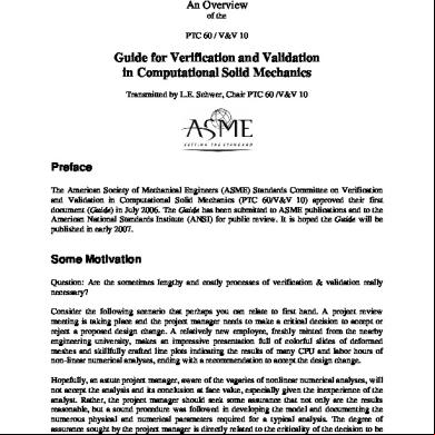
The Model Development Section The processes of verification & validation start, and end, with modeling and models, for it is a computational model we seek to & validate for making predictions within the domain of intended use of the model. Three types of models, from the general to the specific, are described. The logic flow from the most general Conceptual, to Mathematical, to the most specific Computational Model, is illustrated in Figure 1.

Figure 1 The path from Conceptual to Computational Model. (Guide Figure)

Before modeling begins, a reality of interest is identified, i.e. what is the physical system to be modeled. The reality of interest is typically described in the problem statement presented to the analyst, e.g. “We need to know the wing tip deflection of the ABC experimental aircraft under a distributed load of X Newtons/meter,” in this case the reality of interest is the aircraft wing. The most general form of the model addressed in the Guide is the Conceptual Model – “the collection of assumptions and descriptions of physical processes representing the solid mechanics behavior of the reality of interest from which the mathematical model and validation experiments can be constructed.” Continuing the aircraft wing example, the conceptual model could be a cantilever beam of variable cross section made of a laminated composite material, and loaded uniformly along the length. With the Conceptual Model defined, the analyst next defines the Mathematical Model – “The mathematical equations, boundary values, initial conditions, and modeling data needed to describe the conceptual model.” For the aircraft wing example, the analyst might select a Bernoulli-Euler beam theory with fixed-free boundary conditions, i.e.

5

Reprinted by permission of The American Society of Mechanical Engineers. All rights reserved.

⎡ EI ( x ) y′′⎤′′ = w ( x ) ⎣ ⎦

0< x< L

y ( 0 ) = y′ ( 0 ) = y′′ ( L ) = y′′′ ( L ) = 0

The variable cross section geometry of the wing is reflected in the function I ( x ) , for simplicity in this example an elastic material response is assumed, and w ( x ) = constant , represents the uniform load along the span. The final model in the sequence is the Computational Model – “The numerical implementation of the mathematical model, usually in the form of numerical discretization, solution algorithm, and convergence criteria.” This is the stage of modeling most familiar to numerical analysts, as this is where the analyst forms the “input file” used to describe the particulars of the model in the numerical solution software (code) interprets as the model to be solved. At this point the computational model can be exercised (run) and the results compared to available experimental data for validation of the model. It is frequently the case that the results do not compare as favorably as requested in the original problem statement. Assuming a high degree of confidence in the experimental data, the analyst has two basic choices for revising the model: changing the model form or calibrating model parameters. Changing the model form can apply to either the Conceptual or Mathematical model. As an example of a change in the Conceptual model, perhaps the fixed-end cantilever beam assumption was too restrictive and this boundary condition needs to be replaced with a deformable constraint to reflect the wing’s attachment to the fuselage. An example of a change in the Mathematical Model is perhaps the long-and-slender beam assumptions of Bernoulli-Euler beam theory are deemed inappropriate and a Timoshenko beam theory is adopted as the revised Mathematical Model. Perhaps the most misunderstood, and thus most abused, form of model revision is model Calibration – “the process of adjusting physical modeling parameters in the computational model to improve agreement with experimental data.” A trivial example of calibration is the selection of Young’s modulus for a linear elastic constitutive model based on laboratory uniaxial stress data. For the present aircraft wing example, assume it was decided to revise the conceptual model and include a flexible boundary condition to replace the fixed-end assumption. The analyst is then faced with replacing a very complex connection of wing-to-fuselage with a simplified equivalent shear and moment resistance for a beam model. One approach could be to construct a laboratory model of the connection and measure the shear and moment resistance. A separate computational model would be constructed of this laboratory experiment, and the shear and moment resistance calibrated to the laboratory results. These end-reaction calibration values would then be used in the revised mathematical model of the wing, and validation comparisons revisited. It is important to note that the model used in the validation comparison was not calibrated to the validation data, as this results in a calibrated rather than validated model. Rather a sub-system calibration experiment was designed and executed to determine the unknown model parameters.

6

Reprinted by permission of The American Society of Mechanical Engineers. All rights reserved.

The Introduction Section With the above three types of models described, i.e. Conceptual, Mathematical, and Computational, the concepts of verification & validation, and how they fit into an overall V&V Plan, are described. Beginning with the definitions of verification and validation: •

Verification: The process of determining that a computational model accurately represents the underlying mathematical model and its solution.

•

Validation: The process of determining the degree to which a model is an accurate representation of the real world from the perspective of the intended uses of the model.

A careful examination of the verification definition indicates there are two fundamental parts of verification: 1 Code Verification – establish confidence, through the collection of evidence, that the mathematical model and solution algorithms are working correctly. 2 Calculation Verification - establish confidence, through the collection of evidence, that the discrete solution of the mathematical model is accurate. Neither part of verification addresses the question of the adequacy of the selected Conceptual and Mathematical models for representing the reality of interest. Answering this question is the domain of validation, i.e. are the mechanics (physics) included in the Conceptual and Mathematical models sufficient for answering the questions in the problem statement. Put most simply, verification is the domain of mathematics and validation is the domain of physics. The manner in which the mathematics and physics interact in the V&V process is illustrated in the flow chart shown in Figure 2. After the selection of the Conceptual model, the V&V process has two branches: the left branch contains the modeling elements and the right branch the physical testing (experimental) elements. This figure is intentionally designed to illustrate the paramount importance of physical testing in the V&V process, as ultimately, it is only through physical observations (experimentation) that assessments about the adequacy of the selected Conceptual and Mathematical models for representing the reality of interest can be made. Close cooperation among modelers and experimentalist is required during all stages of the V&V process, until the experimental outcomes are obtained. Close cooperation is required because the two groups will have quite different views of the Conceptual model, i.e. the mathematical and physical model will be

7

Reprinted by permission of The American Society of Mechanical Engineers. All rights reserved.

different. As an example consider the fixed-end (clamped) boundary for the aircraft wing illustration. Mathematically this boundary condition is quite easy to specify, but in the laboratory there is no such thing as a ‘clamped’ boundary. In general, some parts of the Conceptual model will be relatively easy to include in either the mathematical or physical model, and others more difficult. A dialogue between the modelers and experimentalist is critical to resolve these differences. To aid in this dialogue, the ‘cross-talk’ activity labeled as “Preliminary Calculations” in Figure 2 is intended to emphasize the goal that both numerical modelers and experimentalist attempt to model the same Conceptual model. Of equal importance is the idea that the experimental outcomes should not be revealed to the modelers until they have completed the simulation outcomes. The chief reason for segregation of the outcomes is to enhance the confidence in the model’s predictive capability. When experimental outcomes are made available to modelers prior to establishing their simulation outcomes, the human tendency is to ‘tune’ the model to the experimental outcomes to produce a favorable comparison. This tendency decreases the level of confidence in the model’s ability to predict, and moves the focus to the model’s ability to mimic the provided experimental outcomes. Lastly, the role of uncertainty quantification (UQ), again for both modelers and experimentalists, is emphasized. It is common to perform more than one experiment and produce somewhat different results. It is the role of UQ to quantify “somewhat” in a meaningful way. Similarly, every computation involves both numerical and physical parameters that have ranges, and likely distributions, of values. Uncertainty quantification techniques attempt to quantify the affect of these parameter variations on the simulation outcomes.

8

Reprinted by permission of The American Society of Mechanical Engineers. All rights reserved.

Figure 2 Verification & Validation activities and outcomes. (Guide Figure)

Figure 2 can also serve as the starting point for forming a V&V Plan, i.e. what are the goals and expected outcomes of the V&V effort and how will the available be resources be allocated. Critical assessment of the resource allocation will often affect the goals of a V&V Plan, but it is better to have such an estimate of this impact before embarking on a V&V effort, than to come to this realization after the resources have been expended without a V&V Plan. The three key elements of the V&V Plan that will help in estimating the resource allocations are: 1 2

System Response Features – the features of interest to be compared and how they are to be compared (metrics). Validation Testing – set of experiments for which the model’s predictive capability is to be demonstrated for the model to be accepted for its intended use.

9

Reprinted by permission of The American Society of Mechanical Engineers. All rights reserved.

3

Accuracy Requirements - specification of accuracy requirements allows the “acceptable agreement” question to be answered quantitatively.

The V&V Plan is of paramount importance to the V&V process. It is the basis for developing the models, assessing the models, and establishes the criteria for accepting the models as suitable for making predictions. Simply put, the specification in the V&V Plan answers the question “What is a validated model?” Finally, the role of documentation throughout the V&V planning process cannot be over emphasized. Eventually the body of evidence comprising the V&V process will need to be presented to an appropriate authority, e.g. management, for their evaluation and subsequent decision-making process. The documentation should try to anticipate and provide answers to the questions raised by such an authority. The documentation also has potential value in the future, e.g. when decisions are revisited or when past knowledge needs to be reused or built upon.

The Verification Section The Guide emphasizes that Verification must precede Validation. The logic is that attempting to validate a model using a code that may still contain (serious) errors can lead to a false conclusion about the validity of the model. As mentioned above, there are two fundamental parts of verification: 1

Code Verification – establish confidence, through the collection of evidence, that the mathematical model and solution algorithms are working correctly. 2 Calculation Verification - establish confidence, through the collection of evidence, that the discrete solution of the mathematical model is accurate.

Code Verification In general, Code Verification is the domain of software developers who hopefully use modern Software Quality Assurance techniques along with testing of each released version of the software. s of software also share in the responsibility for code verification, even though they typically do not have access to the software source. The large number of software s, typical of most commercial codes, provides a powerful potential code verification capability, if it is used wisely by the code developers. Among the code verification techniques, the most popular method is to compare code outputs with analytical solutions; this type of comparison is the mainstay of regression testing. Unfortunately, the complexity of most available analytical solutions pales compared to even rather routine applications of most commercial software. One code verification method with the potential to greatly expand the number and complexity of analytical solutions is what is termed in the V&V literature as manufactured solutions.

10

Reprinted by permission of The American Society of Mechanical Engineers. All rights reserved.

The basic concept of a manufactured solution is deceptively simple. Given a partial differential equation (PDE), and a code that provides general solutions of that PDE, an arbitrary solution to the PDE is manufactured, i.e. made up, then substituted into the PDE along with associated boundary and initial condition, also manufactured. The result is a forcing function (right-hand side) that is the exact forcing function to reproduce the originally selected (manufactured) solution. The code is then subjected to this forcing function and the numerical results compared with the manufactured solution. If the code is error free the two solutions should agree. As an illustration of a manufactured solution, consider again the ordinary differential equation (ODE) for a beam given previously in the Model Development section,

EIy IV = w ( x ) where for simplicity of this illustration a constant cross section has been assumed. The following manufactured solution is proposed:

y ( x ) = A sin

αx

⎛x⎞ + B exp ⎜ ⎟ + C L ⎝L⎠

Where the four constants, i.e. A, α , B, C , are determined from the boundary conditions. Substitution of the manufactured solution into the ODE results in the expression for the forcing function w ( x ) as 4 w( x) αx B ⎛α ⎞ ⎛x⎞ = A ⎜ ⎟ sin + 4 exp ⎜ ⎟ EI L L ⎝L⎠ ⎝ L⎠

The above forcing function would be prescribed as input to the discrete beam element code, and the code’s discrete solution for y ( x ) compared with the selected manufactured solution.

Calculation Verification The above illustration of a manufactured solution used as part of code verification is only half of the verification effort. The other half is what is termed calculation verification, or estimating the errors in the numerical solution due to discretization. Calculation verification, of necessity, is performed after code verification, so that the two error types are not confounded. In the above beam example, a poor comparison of the numerical and analytical solutions would tend to indicate an error in the numerical algorithm. However, any comparison of the numerical and analytical results will contain some error, as the discrete solution, by definition, is only an approximation of the analytical solution. So the goal of calculation verification is to estimate the amount of error in the comparison that can be attributed to the discretization.

11

Reprinted by permission of The American Society of Mechanical Engineers. All rights reserved.

The discretization error is most often estimated by comparing numerical solutions at two more discretizations (meshes) with increasing mesh resolution, i.e. decreasing element size. The objective of this mesh-to-mesh comparison is to determine the rate of convergence of the solution. In the above beam example, if the numerical algorithm for integrating the ODE was the trapezoidal rule, then the error in the numerical solutions should converge at a rate proportion to the square of the mesh size, i.e. second-order convergence for the trapezoidal rule. The main responsibility for Calculation Verification rests with the analyst, or of the software. While it is clearly the responsibility of the software developers to assure their algorithms are implemented correctly, they cannot provide any assurance that a -developed mesh is adequate to obtain the available algorithmic accuracy, i.e. large solution errors due to use of an coarse (unresolved) mesh are attributable to the software . The lack of mesh-refinement studies in solid mechanics may be the largest omission in the verification process. This is particularly distressing, since it is relatively easy to remedy.

The Validation Section The validation process has the goal of assessing the predictive capability of the model. This assessment is made by comparing the predictive results of the model with validation experiments. If these comparisons are satisfactory, the model is deemed validated for its intended use, as stated in the V&V Plan. There is perhaps a subtle point here to be emphasized. The original reason for developing a model was to make predictions for applications of the model where no experimental data could, or would, be obtained. However, in the V&V Plan it was agreed that if the model could adequately predict some related, and typically simpler, instances of the intended use, where experimental data would be obtained, then the model would be validated to make predictions beyond the experimental data for the intended use. Simply put, if the model es the tests in the V&V Plan, then it can be used to make the desired predictions with confidence. The V&V Plan is of paramount importance to the V&V process. When it is said that the model is validated for the intended use, it is not the just the Computational model, which likely will have to change for the predictions of interest, but the Mathematical and Conceptual models upon which the Computation model was built that have been validated. It is through the validation of the Conceptual model that confidence is gained that the correct physics (mechanics) were included in the model development. The key components of the validation process are the: • •

Validation Experiments – experiments performed expressly for the purpose of validating the model. Accuracy Assessment – quantifying how well the experimental and simulation outcomes compare.

The goal of a validation experiment is to be a physical realization of an initial boundary value problem, since an initial boundary value problem is what the computational model was

12

Reprinted by permission of The American Society of Mechanical Engineers. All rights reserved.

developed to solve. Most existing experiments do not meet the requirements of a validation experiment, as they were typically performed for purposes other than validation. Certainly appropriate existing experimental data should be used in the validation process, but the resulting confidence in the model’s ability to make predictions, based on these experimental results, is diminished, relative to validation experiments. The reduced confidence arises from the necessity of an analyst needing to select physical and numerical parameters required for the model that were left undefined in the experiment. As an example, an experiment may report that a steel plate was tested and the steel used was designated A36 steel, indicating the manufacture’s minimum specification for a yield strength of 36,000 psi. In fact the yield strength of the specimen tested could be significant greater than that minimum. The important qualities of a validation experiment include: • •

•

Redundancy of the Data – repeat experiments to establish experimental variation. ing Measurements - not only are measurements of the important system response quantities of interest recorded, but other ing measurements are recorded. An example would be to record the curvature of a beam to a strain gauge measurement. Uncertainty Quantification - errors are usually classified as being either random error (precision) or systematic error (bias).

Once the experimental and simulation outcomes are obtained, the accuracy assessment phase of the validation process can begin. If possible, the comparison of the experimental and simulation outcomes should be made by an interested third party, as this helps to remove a bias that favors either the experimental or the simulation results. In addition to deciding what response quantities should be compared, the V&V Plan should state how the quantities are to be compared. Validation metric is the term used describe the comparison of validation experiment and simulation outcomes. These metrics can range from simple binary metrics, e.g. was the material’s yield strength exceeded, to more complex comparisons involving magnitude and phase difference in wave forms, e.g. deceleration history in a vehicle crash. Whatever the form of the validation metric, the result should be a quantitative assessment of the agreement between the experiment and simulation. Hopefully, this quantification will also include an estimate of the variability in the agreement and a confidence statement about the variability, e.g. the relative error between the experiment and simulations was 18% plus or minus 6% with a 85% confidence level. This three-part comparative statement is provided to the decision maker, along with all the ing V&V documentation, to aide in their decision making process about the validity of the model for the intended use.

The Conclusion Section Some of the remaining important V&V activities requiring guidance from the community: •

Verification – this ‘poor’ sister of validation needs more attention from the V&V research community. Reliance on regression testing for code verification provides 13

Reprinted by permission of The American Society of Mechanical Engineers. All rights reserved.

• • • • •

minimal confidence when using today’s complex multi-physics and multi-scale software. Methods, and their implementation as tools, for verification of increasing software complexity are needed. Quantification of the Value of V&V – if program managers are asked to spend resources on V&V, they needed some measure of the value they are receiving for the resources expended. Incomplete V&V – if the V&V process is terminated before a successful conclusion, what is the best path forward for decision maker? Validation Experimentation – most experiments consume large amounts of resources3, the value of these experiments to the V&V process needs to be quantified to enable decision makers to appropriately allocate resources for this important activity. Uncertainty Quantification – meaningful comparisons of simulations with experiments requires an estimate of the uncertainty in both sets of results, and a comparative assessment of these two uncertain outcomes. Predictive Confidence – when validated models are applied beyond the limited range of validation experiments, how can the confidence in these results be quantified?

Committee Roster for PTC 60/V&V 10 The following is a list of the ASME Committee on Verification & Validation in Computational Solid Mechanics who participated in writing, and voting approval, of the Guide.

OFFICERS L. E. Schwer, Chair H. U. Mair, Vice Chair R. L. Crane, Secretary COMMITTEE PERSONNEL M. C. Anderson, Los Alamos National Laboratory J. A. Cafeo, General Motors Corporation R. L. Crane, The American Society of Mechanical Engineers S. W. Doebling, Los Alamos National Laboratory J. H. Fortna, ANSYS M. E. Giltrud, Defense Threat Deduction Agency J. K. Gran, SRI International T. K. Hasselman, Acta Inc. H. M. Kim, Boeing R. W. Logan, Lawrence Livermore National Laboratory H. U. Mair, Institute for Defense Analyses A. K. Noor, Old Dominion University 3

Often equally large amounts of resources are consumed by the corresponding modeling process.

14

Reprinted by permission of The American Society of Mechanical Engineers. All rights reserved.

W. L. Oberkampf, Sandia National Laboratories J. T. Oden , University of Texas D. K. Pace, Consultant T. Paez, Sandia National Laboratories A. B. Pifko, Consultant L. Proctor, MSC Software J. N. Reddy, Texas A & M University P. J. Roache, Consultant L. E. Schwer, Schwer Engineering P. E. Senseny, Consultant M. S. Shephard, Rensselaer Polytechnic Institute D. A. Simons, Northrop Grumman B. H. Thacker, Southwest Research Institute T. G. Trucano, Sandia National Laboratories R. J. Yang, Ford Motor Company Y. Zhao, St. Jude Medical

The Committee acknowledges the contributions of the following individuals associated with the Committee: G. Gray, Former Member, Los Alamos National Laboratories F. Hemez, Alternate, Los Alamos National Laboratories R. Lust, Alternate, General Motors Corporation C. Nitta, Alternate, Lawrence Livermore National Laboratory V. Romero, Alternate, Sandia National Laboratories J. M. Burns, Liaison Member, Burns Engineering W. G. Steele, Jr., Liaison Member, Mississippi State University

15