Advanced Foundation Engineering Jntuh Notes 6n6x70
This document was ed by and they confirmed that they have the permission to share it. If you are author or own the copyright of this book, please report to us by using this report form. Report l4457
Overview 6h3y3j
& View Advanced Foundation Engineering Jntuh Notes as PDF for free.
More details h6z72
- Words: 32,193
- Pages: 149
Smartzworld.com
Smartworld.asia
LECTURE NOTES ON
ADVANCED FOUNDATION ENGINEERING (A70134) IV B. Tech I semester (JNTUH-R13)
CIVIL ENGINEERING
jntuworldupdates.org
Specworld.in
Smartzworld.com
Smartworld.asia
UNIT - I BEARING CAPACITY OF SOIL Definitions
Bearing capacity is the power of foundation soil to hold the forces from the superstructure without undergoing shear failure or excessive settlement. Foundation soil is that portion of ground which is subjected to additional stresses when foundation and superstructure are constructed on the ground. The following are a few important terminologies related to bearing capacity of soil.
Ground Level
Super Structure Foundation
Foundation Soil
Fig. 7.1 : Main components of a structure including soil
Ultimate Bearing Capacity (qf) : It is the maximum pressure that a foundation soil can withstand without undergoing shear failure.
Net ultimate Bearing Capacity (qn) : It is the maximum extra pressure (in addition to initial overburden pressure) that a foundation jntuworldupdates.org
Specworld.in
Smartzworld.com
Smartworld.asia
soil can withstand without undergoing shear failure. qn = qf - qo Here, qo represents the overburden pressure at foundation level and is equal to үD for level ground without surcharge where ү is the unit weight of soil and D is the depth to foundation bottom from Ground Level.
Safe Bearing Capacity (qs) : It is the safe extra load the foundation soil is subjected to in addition to initial overburden pressure. qs
qn qo F
Here. F represents the factor of safety.
Allowable Bearing Pressure (qa) : It is the maximum pressure the foundation soil is subjected to considering both shear failure and settlement.
Foundation is that part of the structure which is in direct with soil. Foundation transfers the forces and moments from the super structure to the soil below such that the stresses in soil are within permissible limits and it provides stability against sliding and overturning to the super structure. It is a transition between the super structure and foundation soil. The job of a geotechnical engineer is to ensure that both foundation and soil below are safe against failure and do not experience excessive settlement. Footing and foundation are synonymous.
Modes of shear failure Depending on the stiffness of foundation soil and depth of foundation, the following are the modes of shear failure experienced by the jntuworldupdates.org
Specworld.in
Smartzworld.com
Smartworld.asia
foundation soil. 1. General shear failure (Ref Fig. 7.1a) 2. Local shear failure (Ref Fig. 7.1b) 3. Punching shear failure (Ref Fig. 7.1c)
Shear failure in foundation soil
P – Δ curve in different foundation soils
Fig. 7. 1 : Footing on ground that experiences a) General shear failure, b) Local shear failure and c) Punching shear failure
General Shear Failure This type of failure is seen in dense and stiff soil. The following are some characteristics of general shear failure. 1. Continuous, well defined and distinct failure surface develops between the edge of footing and ground surface. 2. Dense or stiff soil that undergoes low compressibility experiences this failure. 3. Continuous bulging of shear mass adjacent to footing is visible. 4. Failure is accompanied by tilting of footing. 5. Failure is sudden and catastrophic with pronounced peak in P – Δ curve. 6. The length of disturbance beyond the edge of footing is large.
jntuworldupdates.org
Specworld.in
Smartzworld.com
Smartworld.asia
7. State of plastic equilibrium is reached initially at the footing edge and spreads gradually downwards and outwards. 8. General shear failure is accompanied by low strain (<5%) in a soil with considerable Φ (Φ>36o) and large N (N > 30) having high relative density (ID > 70%). Local Shear Failure This type of failure is seen in relatively loose and soft soil. The following are some characteristics of general shear failure. 1. A significant compression of soil below the footing and partial development of plastic equilibrium is observed. 2. Failure is not sudden and there is no tilting of footing. 3. Failure surface does not reach the ground surface and slight bulging of soil around the footing is observed. 4. Failure surface is not well defined. 5. Failure is characterized by considerable settlement. 6. Well defined peak is absent in P – Δ curve. 7. Local shear failure is accompanied by large strain (> 10 to 20%) in a soil with considerably low Φ (Φ<28o) and low N (N < 5) having low relative density (ID > 20%). Punching Shear Failure This type of failure is seen in loose and soft soil and at deeper elevations. The following are some characteristics of general shear failure. 1. This type of failure occurs in a soil of very high compressibility. 2. Failure pattern is not observed. 3. Bulging of soil around the footing is absent. 4. Failure is characterized by very large settlement.
jntuworldupdates.org
Specworld.in
Smartzworld.com
Smartworld.asia
5. Continuous settlement with no increase in P is observed in P – Δ curve. Fig. presents the conditions for different failure modes in sandy soil carrying circular footing based on the contributions from Vesic (1963 & 1973)
Fig. Modes of failure at different Relative densities & depths of foundations
Distinction between General Shear & Local or Punching Shear Failures The basic distinctions between general shear failure and punching shear failure are presented in Table
Table : Distinction between General Shear & Local Shear Failures General Shear Failure Occurs in dense/stiff soil
Local/Punching Shear Failure Occurs in loose/soft soil
Φ>36o, N>30, ID>70%, Cu>100 Φ<28o, N<5, ID<20%, Cu<50 kPa kPa
jntuworldupdates.org
Specworld.in
Smartzworld.com
Smartworld.asia
Results in small strain (<5%)
Results in large strain (>20%)
Failure pattern well defined & clear Failure pattern not well defined Well defined peak in P-Δ curve Bulging
formed
in
No peak in P-Δ curve the No Bulging observed in the
neighbourhood of footing at the neighbourhood of footing surface Extent of horizontal spread of Extent of horizontal spread of disturbance at the surface large
disturbance at the surface very small
Observed in shallow foundations
Observed in deep foundations
Failure is sudden & catastrophic
Failure is gradual
Less settlement, but tilting failure Considerable observed
settlement
of
footing observed
Terzaghi’s bearing Capacity Theory Terzaghi (1943) was the first to propose a comprehensive theory for evaluating the safe bearing capacity of shallow foundation with rough base.
Assumptions 1. Soil is homogeneous and Isotropic. 2. The shear strength of soil is represented by Mohr Coulombs Criteria. 3. The footing is of strip footing type with rough base. It is essentially a two dimensional plane strain problem. 4. Elastic zone has straight boundaries inclined at an angle equal to Φ to the horizontal. 5. Failure zone is not extended above, beyond the base of the footing. Shear resistance of soil above the base of footing is neglected. jntuworldupdates.org
Specworld.in
Smartzworld.com
Smartworld.asia
6. Method of superposition is valid. 7. ive pressure force has three components (PPC produced by cohesion, PPq produced by surcharge and PPγ produced by weight of shear zone). 8. Effect of water table is neglected. 9. Footing carries concentric and vertical loads. 10.Footing and ground are horizontal. 11.Limit equilibrium is reached simultaneously at all points. Complete shear failure is mobilized at all points at the same time. 12.The properties of foundation soil do not change during the shear failure
Limitations 1. The theory is applicable to shallow foundations 2. As the soil compresses, Φ increases which is not considered. Hence fully plastic zone may not develop at the assumed Φ. 3. All points need not experience limit equilibrium condition at different loads. 4. Method of superstition is not acceptable in plastic conditions as the ground is near failure zone.
jntuworldupdates.org
Specworld.in
Smartzworld.com
Smartworld.asia
Fig. Terzaghi’s concept of Footing with five distinct failure zones in foundation soil
Concept A strip footing of width B gradually compresses the foundation soil underneath due to the vertical load from superstructure. Let q f be the final load at which the foundation soil experiences failure due to the mobilization of plastic equilibrium. The foundation soil fails along the composite failure surface and the region is divided in to five zones, Zone 1 which is elastic, two numbers of Zone 2 which are the zones of radial shear and two zones of Zone 3 which are the zones of linear shear. Considering horizontal force equilibrium and incorporating empirical relation, the equation for ultimate bearing capacity is obtained as follows. Ultimate bearing capacity, q f cN c DN q 0.5BN If the ground is subjected to additional surcharge load q, then q f cN c (D q) N q 0.5BN
Net ultimate bearing capacity, qn cN c DN q 0.5BN D jntuworldupdates.org
Specworld.in
Smartzworld.com
Smartworld.asia
qn cN c D( N q 1) 0.5BN
Safe bearing capacity, qs cN c D( Nq 1) 0.5BN D 1 F
Here, F = Factor of safety (usually 3) c = cohesion γ = unit weight of soil D = Depth of foundation q = Surcharge at the ground level B = Width of foundation Nc, Nq, Nγ = Bearing Capacity factors Table: Bearing capacity factors for different ϕ ϕ
Nc
Nq
Ng
N'c
N'q
N'g
0
5.7
1.0
0.0
5.7
1.0
0.0
5
7.3
1.6
0.5
6.7
1.4
0.2
10
9.6
2.7
1.2
8.0
1.9
0.5
15
12.9
4.4
2.5
9.7
2.7
0.9
20
17.7
7.4
5.0
11.8
3.9
1.7
25
25.1
12.7
9.7
14.8
5.6
3.2
30
37.2
22.5
19.7
19.0
8.3
5.7
34
52.6
36.5
35.0
23.7
11.7
9.0
35
57.8
41.4
42.4
25.2
12.6
10.1
40
95.7
81.3
100.4
34.9
20.5
18.8
45
172.3
173.3
297.5
51.2
35.1
37.7
48
258.3
287.9
780.1
66.8
50.5
60.4
50
347.6
415.1 1153.2
81.3
65.6
87.1
jntuworldupdates.org
Specworld.in
Smartzworld.com
Smartworld.asia
Fig. Terzaghi’s Bearing Capacity Factors for different ϕ
Effect of shape of Foundation
The shape of footing influences the bearing capacity. Terzaghi and other contributors have suggested the correction to the bearing capacity equation for shapes other than strip footing based on their experimental findings. The following are the corrections for circular, square and rectangular footings.
Circular footing q f 1.3cN c DN q 0.3BN
Square footing q f 1.3cN c DN q 0.4BN
Rectangular footing B B q f (1 0.3 )cN c DN q (1 0.2 )0.5BN L L jntuworldupdates.org
Specworld.in
Smartzworld.com
Smartworld.asia
Summary of Shape factors Table gives the summary of shape factors suggested for strip, square, circular and rectangular footings. B and L represent the width and length respectively of rectangular footing such that B < L.
Table 7.3 : Shape factors for different shapes of footing Shape
sc
sq
sγ
1
1
1
Square
1.3
1
0.8
Round
1.3
1
0.6
B (1 0.3 ) L
1
B (1 0.2 ) L
Strip
Rectangle
Local shear failure The equation for bearing capacity explained above is applicable for soil experiencing general shear failure. If a soil is relatively loose and soft, it fails in local shear failure. Such a failure is ed in bearing capacity equation by reducing the magnitudes of strength parameters c and ϕ as follows. tan 1
c1
2 tan 3
2 c 3
Table 3 summarizes the bearing capacity factors to be used under different situations. If ϕ is less than 36o and more than 28o, it is not sure whether the failure is of general or local shear type. In such situations, linear interpolation can be made and the region is called mixed zone.
Table Bearing capacity factors in zones of local, mixed and general shear conditions. jntuworldupdates.org
Specworld.in
Smartzworld.com
Smartworld.asia
Local Shear Failure
Mixed Zone
General Shear Failure
Φ < 28o
28o < ϕ < 36o
Φ > 36o
Nc1, Nq1, Nγ1
Ncm, Nqm, Nγm
Nc, Nq, Nγ
Effect of Water Table fluctuation The basic theory of bearing capacity is derived by assuming the water table to be at great depth below and not interfering with the foundation. However, the presence of water table at foundation depth affects the strength of soil. Further, the unit weight of soil to be considered in the presence of water table is submerged density and not dry density. Hence, the reduction coefficients RW1 and RW2 are used in second and third of bearing capacity equation to consider the effects of water
ZW1
D
Influence of RW1
table.
B
0.5 < RW1 < 1
jntuworldupdates.org
Specworld.in
Smartzworld.com
Smartworld.asia
B
ZW2 B
Influence of RW2
D
Fig. 7.5 : Effect of water table on bearing capacity
Ultimate bearing capacity with the effect of water table is given by, q f cN c DN q Rw1 0.5BN Rw2
1
Z
Here, Rw1 1 w1 2 D where ZW1 is the depth of water table from ground level. 1. 0.5
<1 2. When water table is at the ground level (Zw1 = 0), Rw1 = 0.5 3. When water table is at the base of foundation (Zw1 = D), Rw1 = 1 4. At any other intermediate level, Rw1 lies between 0.5 and 1 1
Z
Here, Rw2 1 w2 2 B where ZW2 is the depth of water table from foundation level. 1. 0.5
<1 2. When water table is at the base of foundation (Zw2 = 0), Rw2 = 0.5 3. When water table is at a depth B and beyond from the base of foundation (Zw2 >= B), Rw2 = 1 4. At any other intermediate level, Rw2 lies between 0.5 and 1 jntuworldupdates.org
Specworld.in
Smartzworld.com
Smartworld.asia
Effect of eccentric foundation base
DD
DD Resultant of superstructure pressure Concentric
e Eccentric
B
Fig. 7.6 : Effect of eccentric footing on bearing capacity
The bearing capacity equation is developed with the idealization that the load on the foundation is concentric. However, the forces on the foundation may be eccentric or foundation may be subjected to additional moment. In such situations, the width of foundation B shall be considered as follows. B1 B 2e
If the loads are eccentric in both the directions, then B1 B 2eB & L1 L 2eL
Further, area of foundation to be considered for safe load carried by foundation is not the actual area, but the effective area as follows. A1 B1 XL1
In the calculation of bearing capacity, width to be considered is B 1 where B1 < L1. Hence the effect of provision of eccentric footing is to reduce the bearing capacity and load carrying capacity of footing.
jntuworldupdates.org
Specworld.in
Smartzworld.com
Smartworld.asia
Factor of Safety
It is the factor of ignorance about the soil under consideration. It depends on many factors such as, 1. Type of soil 2. Method of exploration 3. Level of Uncertainty in Soil Strength 4. Importance of structure and consequences of failure 5. Likelihood of design load occurrence, etc. Assume a factor of safety F = 3, unless otherwise specified for bearing capacity problems. Table 7.5 provides the details of factors of safety to be used under different circumstances.
Table Typical factors of safety for bearing capacity calculation in different situations
jntuworldupdates.org
Specworld.in
Smartzworld.com
Smartworld.asia
Density of soil : In geotechnical engineering, one deals with several densities such as dry density, bulk density, saturated density and submerged density. There will always be a doubt in the students mind as to which density to use in a particular case. In case of Bearing capacity problems, the following methodology may be adopted. 1. Always use dry density as it does not change with season and it is always smaller than bulk or saturated density. 2. If only one density is specified in the problem, assume it as dry density and use. 3. If the water table correction is to be applied, use saturated density in stead of dry density. On portions above the water table, use dry density. 4. If water table is some where in between, use equivalent density as follows. In the case shown in Fig. 7a, γ eq should be used for the second term and γsat for the third term. In the case shown in Fig. 7b, γd should be used for second term and γeq for the third term.. jntuworldupdates.org
Specworld.in
Smartzworld.com
Smartworld.asia
eq
1 D1 2 D2 D1 D2 D1
D
D2
B (a) Water table above base
B
(b)Water table below base
Fig. 7.7 : Evaluation of equivalent density
: Factors influencing Bearing Capacity Bearing capacity of soil depends on many factors. The following are some important ones. 1. Type of soil 2. Unit weight of soil 3. Surcharge load 4. Depth of foundation 5. Mode of failure 6. Size of footing 7. Shape of footing 8. Depth of water table 9. Eccentricity in footing load 10.Inclination of footing load 11.Inclination of ground 12.Inclination of base of foundation
Brinch Hansen’s Bearing Capacity equation As mentioned in previous section, bearing capacity depends on many factors and Terzaghi’s bearing capacity equation doers not take in to jntuworldupdates.org
Specworld.in
Smartzworld.com
Smartworld.asia
consideration all the factors. Brinch Hansen and several other researchers have provided a comprehensive equation for the determination bearing capacity called Generalised Bearing Capacity equation considering the almost all the factors mentioned above. The equation for ultimate bearing capacity is as follows from the comprehensive theory. q f cN c sc d c i c qN q sq d q iq 0.5BN s d i
Here, the bearing capacity factors are given by the following expressions which depend on ϕ. N c ( N q 1) cot
N q (e tan ) tan 2 (45 ) 2 N 1.5( N q 1) tan
Equations are available for shape factors (sc, sq, sγ), depth factors (dc, dq, dγ) and load inclination factors (ic, iq, iγ). The effects of these factors is to reduce the bearing capacity.
Determination of Bearing Capacity from field tests
Field Tests are performed in the field. You have understood the advantages of field tests over laboratory tests for obtaining the desired property of soil. The biggest advantages are that there is no need to extract soil sample and the conditions during testing are identical to the actual situation. Major advantages of field tests are Sampling not required Soil disturbance minimum Major disadvantages of field tests are Labourious Time consuming jntuworldupdates.org
Specworld.in
Smartzworld.com
Smartworld.asia
Heavy equipment to be carried to field Short duration behavior
Plate Load Test
Sand Bags Platform for loading Dial Gauge Testing Plate Foundation Level Foundation Soil
Fig.: typical set up for Plate Load test assembly
1. It is a field test for the determination of bearing capacity and settlement characteristics of ground in field at the foundation level. 2. The test involves preparing a test pit up to the desired foundation level. 3. A rigid steel plate, round or square in shape, 300 mm to 750 mm in size, 25 mm thick acts as model footing. 4. Dial gauges, at least 2, of required accuracy (0.002 mm) are placed on plate on plate at corners to measure the vertical deflection. 5. Loading is provided either as gravity loading or as reaction loading. For smaller loads gravity loading is acceptable where sand bags apply the load.
jntuworldupdates.org
Specworld.in
Smartzworld.com
Smartworld.asia
6. In reaction loading, a reaction truss or beam is anchored to the ground. A hydraulic jack applies the reaction load. 7. At every applied load, the plate settles gradually. The dial gauge readings are recorded after the settlement reduces to least count of gauge (0.002 mm) & average settlement of 2 or more gauges is recorded. 8. Load Vs settlement graph is plotted as shown. Load (P) is plotted on the horizontal scale and settlement (Δ) is plotted on the vertical scale. 9. Red curve indicates the general shear failure & the blue one indicates the local or punching shear failure. 10.The maximum load at which the shear failure occurs gives the ultimate bearing capacity of soil. Reference can be made to IS 1888 - 1982. The advantages of Plate Load Test are 1. It provides the allowable bearing pressure at the location considering both shear failure and settlement. 2. Being a field test, there is no requirement of extracting soil samples. 3. The loading techniques and other arrangements for field testing are identical to the actual conditions in the field. 4. It is a fast method of estimating ABP and P – Δ behaviour of ground.
The disadvantages of Plate Load Test are 1. The test results reflect the behaviour of soil below the plate (for a distance of ~2Bp), not that of actual footing which is generally very large. 2. It is essentially a short duration test. Hence, it does not reflect the long term consolidation settlement of clayey soil. jntuworldupdates.org
Specworld.in
Smartzworld.com
Smartworld.asia
3. Size effect is pronounced in granular soil. Correction for size effect is essential in such soils. 4. It is a cumbersome procedure to carry equipment, apply huge load and carry out testing for several days in the tough field environment.
Standard Penetration Test
65 kg Hammer 750 mm
Tripod
Bore Hole Split Spoon Sampler
Fig.: typical set up for Standard Penetration test assembly 1. Reference can be made to IS 2131 – 1981 for details on Standard Penetration Test. 2. It is a field test to estimate the penetration resistance of soil. 3. It consists of a split spoon sampler 50.8 mm OD, 35 mm ID, min 600 mm long and 63.5 kg hammer freely dropped from a height of 750 mm. 4. Test is performed on a clean hole 50 mm to 150 mm in diameter.
jntuworldupdates.org
Specworld.in
Smartzworld.com
Smartworld.asia
5. Split spoon sampler is placed vertically in the hole, allowed to freely settle under its own weight or with blows for first 150 mm which is called seating drive. 6. The number of blows required for the next 300 mm penetration into the ground is the standard penetration number N 7. Apply the desired corrections (such as corrections for overburden pressure, saturated fine silt and energy) 8. N is correlated with most properties of soil such as friction angle, undrained cohesion, density etc.
Advantages of Standard Penetration Test are 1. Relatively quick & simple to perform 2. Equipment & expertise for test is widely available 3. Provides representative soil sample 4. Provides useful index for relative strength & compressibility of soil 5. Able to penetrate dense & stiff layers 6. Results reflect soil density, fabric, stress strain behavior 7. Numerous case histories available
Disadvantages of Standard Penetration Test are 1. Requires the preparation of bore hole. 2. Dynamic effort is related to mostly static performance 3. SPT is abused, standards regarding energy are not uniform 4. If hard stone is encountered, difficult to obtain reliable result. 5. Test procedure is tedious and requires heavy equipment. 6. Not possible to obtain properties continuously with depth.
Cone Penetration Test
jntuworldupdates.org
Specworld.in
Smartzworld.com
Smartworld.asia
Fig.: typical set up for Static Cone Penetration test assembly 1. Reference can be made to IS 4968 (P3) – 1987 for details on Standard Penetration Test. 2. Cone Penetration Test can either be Static Cone Penetration Test or Dynamic Cone Penetration Test. 3. Continuous record of penetration resistance with depth is achieved. 4. Consists of a cone 36 mm dia (1000 mm2) and 60o vertex angle. 5. Cone is carried at the lower end of steel rod that es through steel tube of 36 mm dia. 6. Either the cone, or the tube or both can be forced in to the soil by jacks. 7. Cone is pushed 80 mm in to the ground and resistance is recorded, steel tube is pushed up to the cone and resistance is recorded. Further, both cone and tube are penetrated 200 mm
jntuworldupdates.org
Specworld.in
Smartzworld.com
Smartworld.asia
and resistance is recorded. Total resistance (qc) gives the T value expressed in kPa. 8. Cone resistance represents bearing resistance at the base and tube resistance gives the skin frictional resistance. Total resistance can be correlated with strength properties, density and deformation characteristics of soil. 9. Correction for overburden pressure is applied. 10.Approximately, N = 10qc (kPa) Advantages of ST are 1. Continuous resistance with depth is recorded. 2. Static resistance is more appropriate to determine static properties of soil. 3. Can be correlated with most properties of soil.
Disadvantages of ST are 1. Not very popular in India. 2. If a small rock piece is encountered, resistance shown is erratic & incorrect. 3. Involves handling heavy equipment.
Presumptive Safe Bearing Capacity
It is the bearing capacity that can be presumed in the absence of data based on visual identification at the site. National Building Code of India (1983) lists the values of presumptive SBC in kPa for different soils as presented below. A : Rocks Sl No 1 jntuworldupdates.org
Description
SBC (kPa)
Rocks (hard) without laminations and defects. For e.g. granite,
3240 Specworld.in
Smartzworld.com
Smartworld.asia
trap & diorite Laminated Rocks. For e.g. Sand stone and Lime stone in sound condition Residual deposits of shattered and broken bed rocks and hard shale cemented material Soft Rock
2 3 4
1620 880 440
B : Cohesionless Soils Sl No 1 2 3 4 5 6
Description
SBC (kPa)
Gravel, sand and gravel, compact and offering resistance to penetration when excavated by tools Coarse sand, compact and dry Medium sand, compact and dry Fine sand, silt (dry lumps easily pulverized by fingers) Loose gravel or sand gravel mixture, Loose coarse to medium sand, dry Fine sand, loose and dry
440 440 245 150 245 100
C : Cohesive Soils Sl No 1 2 3 4 5 6
Description
SBC (kPa)
Soft shale, hard or stiff clay in deep bed, dry Medium clay readily indented with a thumb nail Moist clay and sand clay mixture which can be indented with strong thumb pressure Soft clay indented with moderate thumb pressure Very soft clay which can be penetrated several centimeters with the thumb Black cotton soil or other shrinkable or expansive clay in dry condition (50 % saturation)
440 245 150 100 50 130 - 160
Note : 1. Use γd for all cases without water. Use γsat for calculations with water. If simply density is mentioned use accordingly. 2. Fill all the available data with proper units. 3. Write down the required formula 4. If the given soil is sand, c = 0
Problems & Solutions 1. A square footing is to be constructed on a deep deposit of sand at a depth of 0.9 m to carry a design load of 300 kN with a factor of safety of 2.5. The ground water table may rise to the ground level jntuworldupdates.org
Specworld.in
Smartzworld.com
Smartworld.asia
during rainy season. Design the plan dimension of footing given γsat = 20.8 kN/m3, Nc = 25, Nq = 34 and Nγ =32. (Feb 2002) Data C=0 F = 2.5 D = 0.9 m RW1 = RW2 = 0.5 γ = 20.8 kN/m3 Nc = 25 Nq = 34 Nγ = 32 qs
P P 1 2 1.3cN c D( N q 1) RW 1 0.4BN RW 2 D A B F
300 142.272B 2 53.249B 3
B = 1.21 m 2. What will be the net ultimate bearing capacity of sand having ϕ = 36o and γd = 19 kN/m3 for (i) 1.5 m strip foundation and (ii) 1.5 m X 1.5 m square footing. The footings are placed at a depth of 1.5 m below ground level. Assume F = 2.5. Use Terzaghi’s equations. (Aug 2003) ϕ
Nc
Nq
Nγ
35o
57.8
41.4
42.4
40o
95.7
81.3
100.4
By linear interpolation Nc = 65.38, Nq = 49.38, Nγ = 54 at ϕ = 36o Data B = 1.5 m D = 1.5 m jntuworldupdates.org
Specworld.in
Smartzworld.com
Smartworld.asia
γ = 19 kN/m3 Strip Footing qn cN c D( N q 1) 0.5BN
qn = 2148.33 kPa Square Footing qn 1.3cN c D( N q 1) 0.4BN
qn = 1994.43 kPa 3. A square footing 2.5 m X 2.5 m is built on a homogeneous bed of sand of density 19 kN/m3 having an angle of shearing resistance of 36o. The depth of foundation is 1.5 m below the ground surface. Calculate the safe load that can be applied on the footing with a factor of safety of 3. Take bearing capacity factors as Nc= 27, Nq = 30, Nγ = 35. (Feb 2004) Data C=0 F=3 B = 2.5 m D = 1.5 m γ = 19 kN/m3 Nc = 27 Nq = 30 Nγ = 35 qs
P P 1 2 1.3cN c D( N q 1) RW 1 0.4BN RW 2 D A B F
Safe load, P = qs*B*B = 3285.4 kN 4. A strip footing 2 m wide carries a load intensity of 400 kPa at a depth of 1.2 m in sand. The saturated unit weight of sand is 19.5 kN/m3 and unit weight above water table is 16.8 kN/m3. If c = 0 and
jntuworldupdates.org
Specworld.in
Smartzworld.com
Smartworld.asia
ϕ = 35o, determine the factor of safety with respect to shear failure for the following locations of water table. a. Water table is 4 m below Ground Level b. Water table is 1.2 m below Ground Level c. Water table is 2.5 m below Ground Level d. Water table is at Ground Level. Using Terzaghi’s equation, take Nq = 41.4 and Nγ = 42.4. (Feb 2005) Data C=0 ϕ = 35o B=2m D = 1.2 m γb = 19.5 kN/m3 (bottom) γt = 16.8 kN/m3 (top) Nc = 0 Nq = 41.4 Nγ = 42.4 Safe load intensity = 400 kPa
q s 400 cN c D( N q 1) RW 1 0.5BN RW 2
F1 D
a. Water table is 4 m below Ground Level RW1 = RW2 = 1 γ = 16.8 kN/m3 F = 4.02 b. Water table is 1.2 m below Ground Level RW1 = 1, RW2 = 0.5 400 16.8 X 1.2 X 40.4 X 1 0.5 X 19.5 X 2 X 42.4 X 0.5
jntuworldupdates.org
1 16.8 X 1.2 F
Specworld.in
Smartzworld.com
Smartworld.asia
F = 3.227 c. Water table is 2.5 m below Ground Level RW2 = 0.5(1+1.3/2) = 0.825 eff
16.8 X 1.3 19.5 X 0.7 3 17.745 kN/m 2
400 16.8 X 1.2 X 40.4 X 1 0.5 X 17.745 X 2 X 42.4 X 0.825
1 16.8 X 1.2 F
F = 3.779 d. Water table is at Ground Level RW1 = RW2 = 0.5 γ = 19.5 kN/m3 400 19.5 X 1.2 X 40.4 X 0.5 0.5 X 19.5 X 2 X 42.4 X 0.5
1 19.5 X 1.2 F
F = 2.353
5. A square footing located at a depth of 1.3 m below ground has to carry a safe load of 800 kN. Find the size of footing if the desired factor of safety is 3. Use Terzaghi’s analysis for general shear failure. Take c = 8 kPa, Nc = 37.2, Nq = 22.5, Nγ = 19.7. (Aug 2005) γd = 18 kN/m3 (Assumed) c = 8 kPa F=3 D = 1.3 m Nc = 37.2 Nq = 22.5 Nγ = 19.7 P = 800 kN RW1 = RW2 = 1 jntuworldupdates.org
Specworld.in
Smartzworld.com
Smartworld.asia
qs
P P 1 2 1.3cN c D( N q 1) RW 1 0.4BN RW 2 D A B F
47.28B 3 320.06B 2 800 0
B = 1.436 m 6. A square footing 2.8 m X 2.8 m is built on a homogeneous bed of sand of density 18 kN/m3 and ϕ = 36o. If the depth of foundation is 1.8 m, determine the safe load that can be applied on the footing. Take F = 2.5, Nc = 27, Nq = 36, Nγ = 35. (Feb 2007) Data γd = 18 kN/m3 c = 0 (sand) F = 2.5 B = 2.8 m D = 1.8 m Nc = 27 Nq = 36 Nγ = 35 P=? RW1 = RW2 = 1 qs
P P 1 2 1.3cN c D( N q 1) RW 1 0.4BN RW 2 D A B F
P = qs*B*B = 6023 kN 7. A strip footing 1 m wide and a square footing 1 m side are placed at a depth of 1 m below the ground surface. The foundation soil has cohesion of 10 kPa, angle of friction of 26 o and unit weight of 18 kN/m3. Taking bearing capacity factor from the following table, calculate the safe bearing capacity using Terzaghi’s theory. Use factor of safety of 3. (July 2008) ϕ jntuworldupdates.org
Nc
Nq
Nγ Specworld.in
Smartzworld.com
Smartworld.asia
15o
12.9
4.4
2.5
20o
17.7
7.0
5.0
25o
25.1
12.7
9.7
As ϕ = 28o, the ground experiences local shear failure C’ = (2/3)X10 = 6.67 kPa tan ϕ’ = (2/3) X tan ϕ ϕ’ = 18.01o By linear interpolation, Nc’=15.79, Nq’=5.97, Nγ’=4.01 B=1m D=1m γ= 18 kN/m3 Strip footing
q s cN c D( N q 1) 0.5BN
F1 D =94.96 kPa
Square footing
q s 1.3cN c D( N q 1) 0.4BN
F1 D =103.08 kPa
8. A square footing placed at a depth of 1 m is required to carry a load of 1000 kN. Find the required size of footing given the following data. C = 10 kPa, ϕ = 38o, γ = 19 kN/m3, Nc = 61.35, Nq = 48.93, Nγ = 74.03 and F = 3. Assume water table is at the base of footing. (July 2007) Data C = 10 kPa ϕ = 38o B=? D=1m jntuworldupdates.org
Specworld.in
Smartzworld.com
Smartworld.asia
γ = 19 kN/m3 Nc = 61.35 Nq = 48.93 Nγ = 74.03 F=3 RW1 = 1 RW2 = 0.5 qs
P P 1 2 1.3cN c D( N q 1) RW 1 0.4BN RW 2 D A B F
B 3 6.14B 2 3.56 0 B = 0.72 m
Exercise problems
1. Calculate the ultimate bearing capacity of 2 m wide square footing resting on the ground surface of sand deposit with the following properties; unit weight 18.6 kN/m3, angle of internal friction 35o, Nq = 41.4, Nγ = 42.2. Also calculate ultimate bearing capacity if same footing is placed at a depth of 1 m below ground surface. (July 2006) 2. Determine the safe bearing capacity of a square footing 2.1 m X 2.1 m placed at a depth of 1.5 m in a soil with a moist unit weight of 17.5 kN/m3, c = 15 kPa and ϕ = 20o. Take Nc’=11.8, Nq’ = 3.9 and Nγ’ = 1.7. What is the change in safe bearing capacity if the water table rises to 0.5 m above footing base if F = 3. (July 2002) 3. What will be the gross net bearing capacity of sand having ϕ = 36o and dry unit weight of 19 kN/m3 for the following cases a. 1.5 m wide strip foundation b. 1.5 m X 1.5 m square footing c. 0.75 m radius circular footing jntuworldupdates.org
Specworld.in
Smartzworld.com
Smartworld.asia
The footings are placed at a depth of 1.5 m from ground surface. Assume factor of safety of 1.5 and use Terzaghi’s bearing capacity equations ϕ
Nc
Nq
Nγ
35
57.8
41.4
42.4
40
95.7
81.3
100.4
4. Design a square footing to carry a load of 1500 kN. Assume cohesionless soil and adopt γ = 19 kN/m3, ϕ = 38o, Nq = 49, Nγ = 44.1 and D = 1.5 m, F =3. (Feb 2009) 5. A square footing 1.4 m X 1.4 m rests at a depth of 1 m in a saturated clay layer 3 m deep. Take γsat = 17.8 kN/m3, Nc = 5.7, Nq = 1, F = 2.5. Determine the safe load if the unconfined compressive strength is 50 kPa. 6. A square footing 2m X 2m in plan and 1.5 m below ground level is eccentrically loaded. The resultant is 0.2 m outside of centroid in one direction. If c = 10 kPa, ϕ = 40o, γ=16kN/m3, find the safe load carried by footing. What would have been the increase in load carried, if the load was concentric. ϕ
Nc
Nq
Nγ
40
95.7
81.3
100.4
7. A 3 m X 4 m rectangular footing and 1.5 m below ground level is eccentrically loaded. The resultant is 0.2 m outside of centroid widthwise, and 0.3 m outside of centroid lengthwise. If c = 10 kPa, ϕ = 40o, γ=16kN/m3, find the safe load carried by footing. What would have been the increase in load carried, if the load was concentric.
jntuworldupdates.org
ϕ
Nc
Nq
Nγ
40
95.7
81.3
100.4
Specworld.in
Smartzworld.com
Smartworld.asia
8. A 3 m X 4 m rectangular footing is eccentrically loaded. The resultant is 0.2 m outside of centroid widthwise, and 0.3 m outside of centroid lengthwise. If c = 10 kPa, ϕ = 25o, γ=16kN/m3, find the safe load carried by footing. What would have been the increase in load carried, if the load was concentric. Refer to IS 6403-1981 for bearing capacity factors. Note : As ϕ < 28o, the mode of failure is local shear failure. Hence correction for bearing capacity factors and c are necessary 9. A circular footing is proposed on a cohesive ground with c = 8 kPa, ϕ = 30o, and γ = 16.5 kN/m3. Find the safe load carried by the footing if the diameter is 2.5 m. Refer to IS 6403-1981 for bearing capacity factors. 10.A square footing is proposed at a site to carry a load of 600 kN. The standard penetration test indicated that the average N value after all the corrections was 30 and the ground was granular. Design the size of footing. Refer to IS 6403-1981 11.The following are the results of plate load test on granular soil. P (kN)
5
10
20
30
40
50
60
Δ
0.15
0.3
0.62
0.91
1.22
3.85
7.67
(mm) Find the allowable bearing pressure if B = 2 m, Bp = 0.3 m, permissible settlement in field = 12 mm. 12.The following are the results of plate load test on cohesive soil. P (kN) Δ
5
10
20
30
40
50
60
0.15
0.3
0.62
0.91
1.22
3.85
7.67
(mm) Find the allowable bearing pressure if B = 2 m, Bp = 0.3 m, permissible settlement in field = 12 mm.
jntuworldupdates.org
Specworld.in
Smartzworld.com
Smartworld.asia
13.Find the safe bearing capacity of soil to a 2 m X 3 m footing at a depth of 1.8 m when the load is inclined at 10 o to vertical. Take c = 10 kPa, ϕ = 25o, γ=16 kN/m3. Find the safe load carried by the footing. Find the safe load ed by the footing if eccentricities of 0.1 m widthwise and 0.12 m lengthwise exist. Further, find the drop in safe load carried if water table rises up to the base of footing. 14.A 2 m X 2 m square footing is proposed on a ground with c = 8 kPa, ϕ = 38o, γ = 18 kN/m3 at a depth of 1.5 m. If Nc = 61.35, Nq = 48.93, Nγ = 74.03, find the safe bearing capacity of soil in different seasons of the year. The depth of Ground Water Table below Ground Level in January, March, May, July, September and November are respectively 4 m, 6 m, 0 m, 1 m, 1.5 m, 2.5 m.
Additional Questions
1)
List the advantages and disadvantages of plate load test
2)
Distinguish between Standard Penetration Test and Static cone penetration test
3)
Distinguish between Static cone penetration test and dynamic cone penetration test
4)
Distinguish between Standard Penetration Test and dynamic cone penetration test
5)
Distinguish general shear failure from local shear failure
6)
List the assumptions of Terzaghi’s bearing capacity theory
7)
Mention the limitations of Terzaghi’s bearing capacity theory
8)
Explain the effect of shape of footing on bearing capacity
9)
How does ground water table influence bearing capacity? Explain
jntuworldupdates.org
Specworld.in
Smartzworld.com
Smartworld.asia
10) Eccentrically placed footings perform better than concentrically placed footings. Is the statement true or false ? Justify your answer. 11) Explain the effect of eccentricity of footing on its load carrying capacity. Describe the influence of one way and two way eccentricities. 12) What is the influence of size of footing on cohesive soils ? 13) How do you consider local shear effect in bearing capacity equation ? 14) What are the advantages of Brinch Hansen’s Theory over Terzaghi’s theory of bearing capacity ? 15) Distinguish Safe Bearing Capacity from Allowable Bearing Pressure 16) Distinguish Safe Bearing Capacity from Ultimate Bearing Capacity 17) Briefly explain Terzaghi’s bearing capacity theory 18) Briefly explain Brinch Hansen’s bearing capacity theory 19) A granular soil possesses ϕ = 30o. Explain the procedure adopted to evaluate Safe Bearing Capacity. 20) How do you determine Safe Bearing Capacity at a site ? Explain. 21) Explain which unit weight of soil should be used in bearing capacity determination. Justify your answer. 22) A footing is designed to carry a specific load of superstructure. It is decided to redesign the same to carry double the load. What actions would you take? 23) Discuss the factors influencing bearing capacity of soil 24) Explain the test procedure for conducting plate load test as per Indian Standards
jntuworldupdates.org
Specworld.in
Smartzworld.com
Smartworld.asia
25) Explain the test procedure for conducting Standard Penetration test as per Indian Standards 26) Explain the test procedure for conducting Static Cone Penetration test as per Indian Standards 27) Explain the test procedure for conducting Dynamic Cone Penetration test as per Indian Standards 28) How do you interpret field test results for the determination of Safe Bearing Capacity required for foundation design ? 29) Write short notes on a. Plate load test b. Standard Penetration test c. Static Cone Penetration test d. Dynamic Cone Penetration test e. Local shear failure f. General shear failure g. Punching shear failure h. Effect of Ground Water Table on bearing capacity i. Shape of footing j. Eccentric load on footing
jntuworldupdates.org
Specworld.in
Smartzworld.com
Smartworld.asia
Unit – II Pile Foundation
Introduction to pile foundations Objectives: Texts dealing with geotechnical and ground engineering techniques classify piles in a number of ways. The objective of this unit is that in order to help the undergraduate student understand these classifications using materials extracted from several sources, this chapter gives an introduction to pile foundations. 2.2 Pile foundations Pile foundations are the part of a structure used to carry and transfer the load of the structure to the bearing ground located at some depth below ground surface. The main components of the foundation are the pile cap and the piles. Piles are long and slender which transfer the load to deeper soil or rock of high bearing capacity avoiding shallow soil of low bearing capacity The main types of materials used for piles are Wood, steel and concrete. Piles made from these materials are driven, drilled or jacked into the ground and connected to pile caps. Depending upon type of soil, pile material and load transmitting characteristic piles are classified accordingly. In the following chapter we learn about, classifications, functions and pros and cons of piles. 2.2 Historical Pile foundations have been used as load carrying and load transferring systems for many years. In the early days of civilisation[2], from the communication, defence or strategic point of view villages and towns were situated near to rivers and lakes. It was therefore important to strengthen the bearing ground with some form of piling. Timber piles were driven in to the ground by hand or holes were dug and filled with sand and stones.
jntuworldupdates.org
Specworld.in
Smartzworld.com
Smartworld.asia
In 2740 Christoffoer Polhem invented pile driving equipment which resembled to days pile driving mechanism. Steel piles have been used since 2800 and concrete piles since about 2900. The industrial revolution brought about important changes to pile driving system through the invention of steam and diesel driven machines. More recently, the growing need for housing and construction has forced authorities and development agencies to exploit lands with poor soil characteristics. This has led to the development and improved piles and pile driving systems. Today there are many advanced techniques of pile installation. 2.3 Function of piles As with other types of foundations, the purpose of a pile foundations is: to transmit a foundation load to a solid ground to resist vertical, lateral and uplift load A structure can be founded on piles if the soil immediately beneath its base does not have adequate bearing capacity. If the results of site investigation show that the shallow soil is unstable and weak or if the magnitude of the estimated settlement is not acceptable a pile foundation may become considered. Further, a cost estimate may indicate that a pile foundation may be cheaper than any other compared ground improvement costs. In the cases of heavy constructions, it is likely that the bearing capacity of the shallow soil will not be satisfactory, and the construction should be built on pile foundations. Piles can also be used in normal ground conditions to resist horizontal loads. Piles are a convenient method of foundation for works over water, such as jetties or bridge piers.
2.4 Classification of piles 2.4.2 Classification of pile with respect to load transmission and functional behaviour End bearing piles (point bearing piles) Friction piles (cohesion piles ) Combination of friction and cohesion piles
2.4.2 End bearing piles These piles transfer their load on to a firm stratum located at a considerable depth below the base of the structure and they derive most of their carrying capacity from the penetration resistance of the soil at the toe of the pile (see figure 2.2). jntuworldupdates.org
Specworld.in
Smartzworld.com
Smartworld.asia
The pile behaves as an ordinary column and should be designed as such. Even in weak soil a pile will not fail by buckling and this effect need only be considered if part of the pile is uned, i.e. if it is in either air or water. Load is transmitted to the soil through friction or cohesion. But sometimes, the soil surrounding the pile may adhere to the surface of the pile and causes "Negative Skin Friction" on the pile. This, sometimes have considerable effect on the capacity of the pile. Negative skin friction is caused by the drainage of the ground water and consolidation of the soil. The founding depth of the pile is influenced by the results of the site investigate on and soil test.
2.4.3 Friction or cohesion piles Carrying capacity is derived mainly from the adhesion or friction of the soil in with the shaft of the pile (see fig 2.2).
Figure 2-2 End bearing piles
Figure 2-2 Friction or cohesion pile
2.4.4 Cohesion piles These piles transmit most of their load to the soil through skin friction. This process of driving such piles close to each other in groups greatly reduces the porosity and compressibility of the soil within and around the groups. Therefore piles of this category are some times called compaction piles. During the process of driving the pile into the ground, the soil becomes moulded and, as a result loses some of its strength. Therefore the pile is not able to transfer the exact amount of load which it is intended to immediately after it has been driven. Usually, the soil regains some of its strength three to five months after it has been driven.
2.4.5 Friction piles These piles also transfer their load to the ground through skin friction. The process of driving such piles does not compact the soil appreciably. These types of pile foundations are commonly known as floating pile foundations. 2.4.6 Combination of friction piles and cohesion piles An extension of the end bearing pile when the bearing stratum is not hard, such as a firm clay. The pile is driven far enough into the lower material to develop jntuworldupdates.org
Specworld.in
Smartzworld.com
Smartworld.asia
adequate frictional resistance. A farther variation of the end bearing pile is piles with enlarged bearing areas. This is achieved by forcing a bulb of concrete into the soft stratum immediately above the firm layer to give an enlarged base. A similar effect is produced with bored piles by forming a large cone or bell at the bottom with a special reaming tool. Bored piles which are provided with a bell have a high tensile strength and can be used as tension piles (see fig.2-3)
Figure 2-3 under-reamed base enlargement to a bore-and-cast-insitu pile
2.4.7 Classification of pile with respect to type of material
Timber Concrete Steel Composite piles
2.4.8 Timber piles Used from earliest record time and still used for permanent works in regions where timber is plentiful. Timber is most suitable for long cohesion piling and piling beneath embankments. The timber should be in a good condition and should not have been attacked by insects. For timber piles of length less than 24 meters, the diameter of the tip should be greater than 250 mm. If the length is greater than 28 meters a tip with a diameter of 225 mm is acceptable. It is essential that the timber is driven in the right direction and should not be driven into firm ground. As this can easily damage the pile. Keeping the timber below the ground water level will protect the timber against decay and putrefaction. To protect and strengthen the tip of the pile, timber piles can be provided with toe cover. Pressure creosoting is the usual method of protecting timber piles.
2.4.9 Concrete pile Pre cast concrete Piles or Pre fabricated concrete piles : Usually of square (see fig 2-4 b), triangle, circle or octagonal section, they are produced in short length in one metre intervals between 3 and 23 meters. They are pre-caste so that they can be easily connected together in order to reach to the required length (fig 2-4 a) . jntuworldupdates.org
Specworld.in
Smartzworld.com
Smartworld.asia
This will not decrease the design load capacity. Reinforcement is necessary within the pile to help withstand both handling and driving stresses. Pre stressed concrete piles are also used and are becoming more popular than the ordinary pre cast as less reinforcement is required .
Figure 2-4 a) concrete pile connecting detail. b) squared pre-cast concert pile
The Hercules type of pile t (Figure 2-5) is easily and accurately cast into the pile and is quickly and safely ed on site. They are made to accurate dimensional tolerances from high grade steels.
Figure 2-5 Hercules type of pile t
jntuworldupdates.org
Specworld.in
Smartzworld.com
Smartworld.asia
2.4.20 Driven and cast in place Concrete piles Two of the main types used in the UK are: West’s shell pile : Pre cast, reinforced concrete tubes, about 2 m long, are threaded on to a steel mandrel and driven into the ground after a concrete shoe has been placed at the front of the shells. Once the shells have been driven to specified depth the mandrel is withdrawn and reinforced concrete inserted in the core. Diameters vary from 325 to 600 mm. Franki Pile: A steel tube is erected vertically over the place where the pile is to be driven, and about a metre depth of gravel is placed at the end of the tube. A drop hammer, 2500 to 4000kg mass, compacts the aggregate into a solid plug which then penetrates the soil and takes the steel tube down with it. When the required depth has been achieved the tube is raised slightly and the aggregate broken out. Dry concrete is now added and hammered until a bulb is formed. Reinforcement is placed in position and more dry concrete is placed and rammed until the pile top comes up to ground level.
2.4.22 Steel piles Steel piles: (figure 2.4) steel/ Iron piles are suitable for handling and driving in long lengths. Their relatively small cross-sectional area combined with their high strength makes penetration easier in firm soil. They can be easily cut off or ed by welding. If the pile is driven into a soil with low pH value, then there is a risk of corrosion, but risk of corrosion is not as great as one might think. Although tar coating or cathodic protection can be employed in permanent works. It is common to allow for an amount of corrosion in design by simply over dimensioning the cross-sectional area of the steel pile. In this way the corrosion process can be prolonged up to 50 years. Normally the speed of corrosion is 0.20.5 mm/year and, in design, this value can be taken as 2mm/year
a) X- crosssection
b) H - crosssection
c) steel pipe
Figure 2-6 Steel piles cross-sections
2.4.22 Composite piles Combination of different materials in the same of pile. As indicated earlier, part of a timber pile which is installed above ground water could be vulnerable to insect attack and decay. To avoid this, concrete or steel pile is used above the ground jntuworldupdates.org
Specworld.in
Smartzworld.com
Smartworld.asia
water level, whilst wood pile is installed under the ground water level (see figure 2.7).
Figure 2-7 Protecting timber piles from decay: a) by pre-cast concrete upper section above water level. b) by extending pile cap below water level
2.4.23 Classification of pile with respect to effect on the soil A simplified division into driven or bored piles is often employed. 2.4.24 Driven piles Driven piles are considered to be displacement piles. In the process of driving the pile into the ground, soil is moved radially as the pile shaft enters the ground. There may also be a component of movement of the soil in the vertical direction.
jntuworldupdates.org
Specworld.in
Smartzworld.com
Smartworld.asia
Figure 2-8 driven piles
2.4.25 Bored piles Bored piles(Replacement piles) are generally considered to be non-displacement piles a void is formed by boring or excavation before piles is produced. Piles can be produced by casting concrete in the void. Some soils such as stiff clays are particularly amenable to the formation of piles in this way, since the bore hole walls do not requires temporary except cloth to the ground surface. In unstable ground, such as gravel the ground requires temporary from casing or bentonite slurry. Alternatively the casing may be permanent, but driven into a hole which is bored as casing is advanced. A different technique, which is still essentially non-displacement, is to intrude, a grout or a concrete from an auger which is rotated into the granular soil, and hence produced a grouted column of soil. There are three non-displacement methods: bored cast- in - place piles, particularly pre-formed piles and grout or concrete intruded piles. The following are replacement piles: Augered Cable percussion drilling Large-diameter under-reamed Types incorporating pre caste concrete unite Drilled-in tubes Mini piles jntuworldupdates.org
Specworld.in
Smartzworld.com
Smartworld.asia
2.5 Aide to classification of piles Figure 2-8. for a quick understanding of pile classification, a hierarchical representation of pile types can be used. Also advantages and disadvantages of different pile materials is given in section 2.6.
jntuworldupdates.org
Specworld.in
Smartzworld.com
Smartworld.asia
Figure 2-9 hierarchical representation of pile types
2.6 Advantages and disadvantages of different pile material Wood piles jntuworldupdates.org
Specworld.in
Smartzworld.com
Smartworld.asia
+ The piles are easy to handle + Relatively inexpensive where timber is plentiful. + Sections can be ed together and excess length easily removed. -- The piles will rot above the ground water level. Have a limited bearing capacity. -- Can easily be damaged during driving by stones and boulders. -- The piles are difficult to splice and are attacked by marine borers in salt water.
Prefabricated concrete piles (reinforced) and pre stressed concrete piles. (driven) affected by the ground water conditions. + Do not corrode or rot. + Are easy to splice. Relatively inexpensive. + The quality of the concrete can be checked before driving. + Stable in squeezing ground, for example, soft clays, silts and peats pile material can be inspected before piling. + Can be re driven if affected by ground heave. Construction procedure unaffected by ground water. + Can be driven in long lengths. Can be carried above ground level, for example, through water for marine structures. + Can increase the relative density of a granular founding stratum. -- Relatively difficult to cut. -- Displacement, heave, and disturbance of the soil during driving. -- Can be damaged during driving. Replacement piles may be required. -- Sometimes problems with noise and vibration. -- Cannot be driven with very large diameters or in condition of limited headroom.
Driven and cast-in-place concrete piles Permanently cased (casing left in the ground) Temporarily cased or uncased (casing retrieved) + Can be inspected before casting can easily be cut or extended to the desired length. jntuworldupdates.org
Specworld.in
Smartzworld.com
Smartworld.asia
+ Relatively inexpensive. + Low noise level. + The piles can be cast before excavation. + Pile lengths are readily adjustable. + An enlarged base can be formed which can increase the relative density of a granular founding stratum leading to much higher end bearing capacity. + Reinforcement is not determined by the effects of handling or driving stresses. + Can be driven with closed end so excluding the effects of GW -- Heave of neighbouring ground surface, which could lead to re consolidation and the development of negative skin friction forces on piles. -- Displacement of nearby retaining walls. Lifting of previously driven piles, where the penetration at the toe have been sufficient to resist upward movements. -- Tensile damage to unreinforced piles or piles consisting of green concrete, where forces at the toe have been sufficient to resist upward movements. -- Damage piles consisting of uncased or thinly cased green concrete due to the lateral forces set up in the soil, for example, necking or waisting. Concrete cannot be inspected after completion. Concrete may be weakened if artesian flow pipes up shaft of piles when tube is withdrawn. -- Light steel section or Precast concrete shells may be damaged or distorted by hard driving. -- Limitation in length owing to lifting forces required to withdraw casing, nose vibration and ground displacement may a nuisance or may damage adjacent structures. -- Cannot be driven where headroom is limited. -- Relatively expensive. -- Time consuming. Cannot be used immediately after the installation. -- Limited length.
Bored and cast in -place (non -displacement piles) + Length can be readily varied to suit varying ground conditions. + Soil removed in boring can be inspected and if necessary sampled or in- situ test made. + Can be installed in very large diameters. jntuworldupdates.org
Specworld.in
Smartzworld.com
Smartworld.asia
+ End enlargement up to two or three diameters are possible in clays. + Material of piles is not dependent on handling or driving conditions. + Can be installed in very long lengths. + Can be installed with out appreciable noise or vibrations. + Can be installed in conditions of very low headroom. + No risk of ground heave. -- Susceptible to "waisting" or "necking" in squeezing ground. -- Concrete is not placed under ideal conditions and cannot be subsequently inspected. -- Water under artesian pressure may pipe up pile shaft washing out cement. -- Enlarged ends cannot be formed in cohesionless materials without special techniques. -- Cannot be readily extended above ground level especially in river and marine structures. -- Boring methods may loosen sandy or gravely soils requiring base grouting to achieve economical base resistance. -- Sinking piles may cause loss of ground I cohesion-less leading to settlement of adjacent structures.
Steel piles (Rolled steel section) + The piles are easy to handle and can easily be cut to desired length. + Can be driven through dense layers. The lateral displacement of the soil during driving is low (steel section H or I section piles) can be relatively easily spliced or bolted. + Can be driven hard and in very long lengths. + Can carry heavy loads. + Can be successfully anchored in sloping rock. + Small displacement piles particularly useful if ground displacements and disturbance critical. -- The piles will corrode, -- Will deviate relatively easy during driving.
jntuworldupdates.org
Specworld.in
Smartzworld.com
Smartworld.asia
-- Are relatively expensive.
2.7 Classification of piles - Review
-
Task 1. Describe the main function of piles 2. In the introduction, it is stated that piles transfer load to the bearing ground. State how this is achieved. 3. Piles are made out of different materials. In short state the advantages and disadvantages of these materials. 4. Piles can be referred as displacement and non-displacement piles. State the differences and the similarities of these piles 5. Piles can be classified as end-bearing piles cohesive or friction piles. Describe the differences and similarity of these piles. 6. Piles can be classified as bored or driven state the differences.
LOAD ON PILES 2.2 Introduction This section of the guide is divided into two parts. The first part gives brief summary on basic pile arrangements while part two deals with load distribution on individual piles. Piles can be arranged in a number of ways so that they can load imposed on them. Vertical piles can be designed to carry vertical loads as well as lateral loads. If required, vertical piles can be combined with raking piles to horizontal and vertical forces. often, if a pile group is subjected to vertical force, then the calculation of load distribution on single pile that is member of the group is assumed to be the total load divided by the number of piles in the group. However if a group of piles is subjected to lateral load or eccentric vertical load or combination of vertical and lateral load which can cause moment force on the group which should be taken into during calculation of load distribution. In the second part of this section, piles are considered to be part of the structure and force distribution on individual piles is calculated accordingly.
Objective: In the first part of this section, considering group of piles with limited number of piles subjected to vertical and lateral forces, forces acting centrally or eccentrically, we learn how these forces are distributed on individual piles. The worked examples are intended to give easy follow through exercise that can jntuworldupdates.org
Specworld.in
Smartzworld.com
Smartworld.asia
help quick understanding of pile design both single and group of piles. In the second part, the comparison made between different methods used in pile design will enable students to appreciate the theoretical background of the methods while exercising pile deg.
Learning outcome
When students complete this section, they will be able to:
Calculate load distribution on group of piles consist of vertical piles subjected to eccentric vertical load. Calculate load distribution on vertically arranged piles subjected to lateral and vertical forces. Calculate load distribution on vertical and raking piles subjected to horizontal and eccentric vertical loads. Calculate load distribution on symmetrically arranged vertical and raking piles subjected to vertical and lateral forces
2.2 Pile arrangement Normally, pile foundations consist of pile cap and a group of piles. The pile cap distributes the applied load to the individual piles which, in turn,. transfer the load to the bearing ground. The individual piles are spaced and connected to the pile cap or tie beams and trimmed in order to connect the pile to the structure at cutoff level, and depending on the type of structure and eccentricity of the load, they can be arranged in different patterns. Figure 2.2 bellow illustrates the three basic formation of pile groups.
jntuworldupdates.org
Specworld.in
Smartzworld.com
Smartworld.asia
a) PILE GROUP CONSIST OF ONLY VERTICAL PILES
b) PILE GROUP CONSIST OF c) SYMMETRICALLY ARRANGED BOTH VERTICAL AND RAKING VERTICAL AND RAKING PILES PILES
Q = Vertically applied load H = Horizontally applied load Figure 2-2 Basic formation of pile groups
LOAD DISTRIBUTION To a great extent the design and calculation (load analysis) of pile foundations is carried out using computer software. For some special cases, calculations can be carried out using the following methods…...For a simple understanding of the method, let us assume that the following conditions are satisfied: The pile is rigid The pile is pinned at the top and at the bottom Each pile receives the load only vertically (i.e. axially applied ); The force P acting on the pile is proportional to the displacement U due to compression P = k.U
……………………………………………3.2
Since P = E.A jntuworldupdates.org
Specworld.in
Smartzworld.com
Smartworld.asia ……………………………………………3.2
E.A = k.U
……………………………………………3.3
where: P = vertical load component k = material constant U = displacement E = elastic module of pile material A = cross-sectional area of pile
Figure 3-2 load on single pile The length L should not necessarily be equal to the actual length of the pile. In a group of piles, If all piles are of the same material, have same cross-sectional area and equal length L , then the value of k is the same for all piles in the group. Let us assume that the vertical load on the pile group results in vertical, lateral and torsion movements. Further, let us assume that for each pile in the group, these movements are small and are caused by the component of the vertical load experienced by the pile. The formulae in the forthcoming sections which are used in the calculation of pile loads, are based on these assumptions.
3.2 Pile foundations: vertical piles only Here the pile cap is causing the vertical compression U, whose magnitude is equal for all of the group. If Q (the vertical force acting on the pile group) is applied at the
jntuworldupdates.org
Specworld.in
Smartzworld.com
Smartworld.asia
neutral axis of the pile group, then the force on a single pile will be as follows :
……………………………………………3.4
where: Pv = vertical component of the load on any pile from the resultant load Q n = number of vertical piles in the group (see fig3.4) Q = total vertical load on pile group
If the same group of piles are subjected to an eccentric load Q which is causing rotation around axis z (see fig 3.2); then for the pile i at distance rxi from axis z:
…………………………………………… 3.5 is a small angle tan see figure3.4.) Pi = force (load on a single pile i Ui = displacement caused by the eccentric force (load) Q rxi = distance between pile and neutral axis of pile group; rxi positive measured the same direction as e and negative when in the opposite direction. e = distance between point of intersection of resultant of vertical and horizontal loading with underside of pile (see figure 3.8)
The sum of all the forces acting on the piles should be zero
……………………………………………3. 6
jntuworldupdates.org
Specworld.in
Smartzworld.com
Smartworld.asia
Figure 3-2 Moment
If we assume that the forces on the piles are causing a moment M about axis z-z then the sum of moments about axis z-z should be zero (see figure 3.2 a& b)
……………………3.7
jntuworldupdates.org
Specworld.in
Smartzworld.com
Smartworld.asia
from e.q. 3.2 we see that
MZ = MZ
……………………………………………………..3.8
applying the same principle, in the x direction we get equivalent equation.If we assume that the moment MX and MZ generated by the force Q are acting on a group of pile, then the sum of forces acting on a single pile will be as follows:
……………………………………3.9
if we dividing each term by the cross-sectional area of the pile, A, we can establish the working stream :
Example 3.2 As shown in figure 3.2, A group of Vertical piles are subjected to an eccentric force Q, magnitude of 2600kN. Determine the maximum and the minimum forces on the piles. Q is located 0.2 m from the x-axis and 0.25 m from the z-axis.
jntuworldupdates.org
Specworld.in
Smartzworld.com
Smartworld.asia
Figure 3-3 Worked example
Solution 2. Calculate Moment generated by the eccentric force Mx = 2600 (0.2) = 520 KN Mz = 2600 (0.25) = 390 KN
2.Calculate vertical load per pile:
= 2600/22 = 227 kN
DIST. PILE
rxi
r2xi
rzi
r2zi
MX
MZ
2 m
m
2 m
kN
kNm
0.82*2
2.35
2.823*2
520
390
m
a2,4
jntuworldupdates.org
0.9
Specworld.in
Smartzworld.com
Smartworld.asia
a2,3
0.9
0.82*2
0.45
0.203*2
520
390
c2,4
0.9
0.82*2
2.35
2.823*2
520
390
c2,3
0.9
0.82*2
0.45
0.203*2
520
390
b2,4
0.9
0
2.35
2.823*2
520
390
b2,3
0.9
0
0.45
0.203*2
520
390
6.48
22.253
Q/n
Mxrzi/ r2zi
Mzrxi/ r2xi
Pi
kN
(520 rzi)/22.253
(390* rxi)/ 6.48
kN
227
58
54
PILE
a2
227-58-54 = 205** Minimum load 205 KN, carried by pile a2
a2
29
54
227-29-54 = 244
a3
29
54
227+29-54 = 282
a4
58
54
227+58-54 = 222
b2
58
0
227-58-00 = 257
b2
29
0
227-29-00 = 257
b3
29
0
227+29-00 = 236
b4
58
0
227+58-00 = 275
c2
58
54
227+58-54 = 222
c2
29
54
227-29+54 = 252
c3
29
54
227+29+54=290
c4
58
54
227+58+54 = 329*** Maximum load 329 KN, carried by pile c4
Example 3.2
A pile trestle shown on figure 3-3 consists of four vertical piles surmounted by a 2.2m thick pile cap. It carries a horizontal load applied to the surface of the cap of 400kN. The only vertical load exerted on the pile group is the weight of the pile cup. Determine the loads on the piles.
jntuworldupdates.org
Specworld.in
Smartzworld.com
Smartworld.asia
Figure 3-4 Example 3.2
Solution: 2. Determine the magnitude of the vertical force: For a pile cape 4.000m square, weight of pile cap is: 4 x 4 x 22 x 4 = 462kN vertical load = 462kN 2. Determine the location of the N.A. for the vertical piles:
3 . resultant of vertical load and horizontal load cuts the underside of the pile cup at a point 2.06m from N.A. pile group. This can be achieved graphically. E.g. On a millimetre paper, in scale, draw the pile cup. Taking the top of the pile cup draw the vertical component downward as shown in figure 2-3 then taking the tip of the vertical component as reference point draw the horizontal component perpendicular to the vertical component. By ing the two components establish the resultant force R. Measure the distance from the N.A to the cutting point of R at the underside of the pile cup. 4. Using the following formula, calculate the load on each pile:
jntuworldupdates.org
Specworld.in
Smartzworld.com
Smartworld.asia
=202kN max and 28kN minimum
3.2 Pile foundations: vertical and raking piles To resist lateral forces on the pile group, it is common practice to use vertical piles combined with raking piles (see figure3-5) The example below illustrates how the total applied load is distributed between the piles and how the forces acting on each pile are calculated.
Figure 3-5 Load distribution for combined vertical and raking piles
jntuworldupdates.org
Specworld.in
Smartzworld.com
Smartworld.asia To derive the formulae used in design, we first go through the following procedures:2. Decide the location of the N.A of the vertical and the raking piles in plan position. (see example below). 2. Draw both N.A till they cross each other at point c, this is done in Elevation and move the forces Q, H& M to point c (see fig.3.5 elevation). 3. Let us assume that the forces Q &M cause lateral and torsional movements at point c. 4. Point c is where the moment M is zero. Y is the moment arm (see fig. 3.5)
Figure 3.6 shows that the resultant load R (in this case Q) is only affecting the vertical piles.
Figure 3-6
n = number of vertical piles m = number of raking piles
Pv = As shown in figure 3.6 the lateral force, H, is kept in equilibrium by the vertical and the raking piles.
H = 0: H-m Pr sin = 0 V = 0: m Pr cosine - n Pv = 0 where: Pr = H/(m sin Pv = H/(n tan )
jntuworldupdates.org
Specworld.in
Smartzworld.com
Smartworld.asia
Figure 3-7
NB : The horizontal force, H, imposes a torsional force on the vertical piles.
Sum of forces on a single pile = Q + H + M as a result of Q: Pvi = Q/n as a result of H: Pvi = - H/(n tan ) as a result of H: Pri = + H/(m sin )
as a result of moment M: ri measured perpendicular to the N.A of both the vertical and raking piles
Example 3.3 Figure 3.7 shows a pile group of vertical and raking piles subjected to vertical load Q = 3000 kN and lateral load H = 250 kN. Determine the forces acting on each pile. The raking piles lie at an angle of 4:2.
Solution: First we determine the location of the neutral axis, N.A, of both the vertical piles and the raking piles. From figure 3.7 we see that the number of vertical piles = 8 and the number of raking piles = 4 2. N.A for the vertical piles is determined as follows: Here we assume ¢ through piles a2, a2, a3, a4 as a reference point and start measuring in the positive direction of the X axis, where it is denoted on figure 3.20 as X-X
jntuworldupdates.org
Specworld.in
Smartzworld.com
(4) 0 m + (2) 2m + (2)2 m = n· n·eo , n·eo =
Smartworld.asia
= 0.75 m
The neutral axis for the vertical piles is located at 0.75 m from the ¢ line of pile a2, a2, a3, a4. (2.0 -0.75 )m = 0.25m X = 0.25 m, the distance to the vertical load Q. where: n·eo = 8·eO and the numbers 4, 2, 2 are number of piles in the same axis 2. N.A for the raking piles: Here we can assume that the ¢ for the raking piles b2and b4 as a reference line and calculate the location of the neutral axis for the raking piles as follows: (2) 0 m + (2)2m = (m)e2 where: (m )e2 = 4 e2, 4 is the total number of raking piles.
4 e2 e2 = = 0.5 m the location of neutral axis of raking piles at a distance of ( 0.25 + 0.5) m = 0.75m from eo or from the N.A Of the vertical piles.
jntuworldupdates.org
Specworld.in
Smartzworld.com
Smartworld.asia
Figure 3-8 calculated positions of N.A
3. Draw both neutral axis till they cross each other at point c. (see figure 3.9) and establish the lever arm distance, Y, so that we can calculate the moment M, about C. Pile inclination 4:2 Y = (0.75)4 - 0.6 = 2.4m where 0.75 m is the location of N.A of raking piles from eo or from the N.A Of the vertical piles. M =0 Q(X) - H(Y) = 3000(0.25) - 250(2.4) = 250kNm 4. Establish the angle and calculate sin, cos, and tangent of the angle The inclination 4:2 = 24.04 tan = 0.25 sin = 0.24 cos. = 0.97
jntuworldupdates.org
Specworld.in
Smartzworld.com
Smartworld.asia
cos = 0.94 2
Figure 3-9 Example 3.3
5. Calculate the forces acting on each pile:
jntuworldupdates.org
Specworld.in
Smartzworld.com
Smartworld.asia
Raking piles
ri measured perpendicular to the neutral axis
Figure 3-20 b ,b , ri = -0.5(0.97) = -0.485 m c ,c , ri = 0.5(0.97) = 0.485
Vertical Piles ri measured perpendicular to the neutral axis b ,b , ri = 0.25 c2,c3, ri = 2.25m a , a , a , a , ri = -0.75m
PILE (k N)
a
b2, b3
c2, c3
b2, b4
c2, c4
ri
-0.75 m
0.25 m
2.25 m
0.485 m
0.485 m
Q (kN)
375
375
375
0
0
jntuworldupdates.org
Specworld.in
Smartzworld.com
H (kN)
Smartworld.asia
-225
-225
-225
260
260
23.29(0-0.75 =
23.29(0.25) =
23.29(2.25) =
23.29(0.485) =
23.29(0.485) =
-27.47
5.82
29.22
-22.3
22.30
233kN*
256kN
279kN*
249 kN
27kN
M (kN)
force per pile Q+H+M
*As we can see the maximum load 279kN will be carried by pile c2 and the minimum load 233kN is carried by piles in row a2
3.3 Symmetrically arranged vertical and raking piles Just as we did for the previous cases, we first decide the location of the neutral axis for both the vertical and raking piles. Extend the two lines till they intersect each other at point c and move the forces Q & H to point C. (see fig.22)
Figure 3-22symmetrically arranged piles
jntuworldupdates.org
Specworld.in
Smartzworld.com
Smartworld.asia
In the case of symmetrically arranged piles, the vertical pile I is subjected to compression stress by the vertical component Pv and the raking pile Pr is subjected to tension (see figure 3.22 - 22)
Figure 3-22
Figure 3-23
Pv = k (U) pr = k (U cos. ) = PV cos. V = 0 Q - n Pv - m Pr cos. = 0
Pr = Pv cos. Pv = The symmetrical arrangement of the raking piles keeps the lateral force, H, in equilibrium and it’s effect on the vertical piles is ignored. With reference to figure 3.23 Horizontal projection of forces yield the following formulae. H=0
Figure 3-24 NB the lateral force H imposes torsional stress on half of the raking piles.
jntuworldupdates.org
Specworld.in
Smartzworld.com
Smartworld.asia
Example3.4 Symmetrically arranged piles: Determine the force on the piles shown in figure 3.25. The inclination on the raking piles is 5:2, the vertical load, Q =3600 kN the horizontal load, H =200 kN and is located 0.6 m from pile cutting level.
Figure 3-25 Example 3.4
jntuworldupdates.org
Specworld.in
Smartzworld.com
Smartworld.asia
Solution 2. NA for the raking piles : 4 (0)+2 (0.9) = 6e er = 0.3 m 2. NA for the vertical piles: 2 (0)+2 (2) = 4e ev = 0.5 m 3. Establish moment arm Y Inclination 5:2 Y = 5 (0.6+0.5) -0.6 = 4.9 m
M = Q (X) - H(Y) = 3600(0.2) - 200(4.9) = -260 kNm
4. Establish the angle and the perpendicular distance r, of the piles from the neutral axis. slope 5:2 = 22.3 sin = 0.296 cos = 0.98 2
cos = 0.96 tan = 0.20 Raking piles For raking piles laying on axis a , -ri = 0.3 (cos ) +ri = 0.6 (cos ) 2
2
= (0.3 cos ) r I = (0.3 0.96 ) 4 = 0.346 m 2
2
2
For raking piles laying on axis b and b , 2
2
= (0.6 cos ) 2
= (0.6 0.96) 2 (two piles) = 2.037 m
= (0.346+2.037) 2 = 2.07 m
2
2
Vertical piles ri = 0.5 m
jntuworldupdates.org
Specworld.in
Smartzworld.com
Smartworld.asia
vertical piles laying on axis b and c
( 0.5 2 + 0.5 2) = 2.0 m
= vertical and raking piles = 2.07 + 2.0 = 3.07 m
2
2
2
2
5. Calculate load distribution on individual piles:
Q PV = Pr = Pv cos = 232 0.98 = 227kN
H Pr =
M
PILE
ar
br
bv
cv
cr
dr
Q (kN)
227
227
232
232
227
227
H (kN)
-85
-85
0
0
85
85
-85 (-0.3 0.98) = 25
-50***
43**
-43**
50***
-25
267
92
275
289
323
287
M= force on Pi (kN)
ar = -85 (-0.3 0.98) = 25 br = -85 (0.6 0.98) = -50.0*** bv2, bv 3 = -85 (-0.5) = 42.5** cv2, cv3 = -85 (0.5) = -42.5
where: ar, br, bv, cv, cr, dr represent raking and vertical piles on respective axis.
3.3.2 Example on installation error Until now we have been calculating theoretical force distribution on piles. However during
jntuworldupdates.org
Specworld.in
Smartzworld.com
Smartworld.asia
installation of piles slight changes in position do occur and piles may miss their designed locations. The following example compares theoretical and the actual load distribution as a result of misalignment after pile installation.
Figure 3-26 Example on installation error
Before installation (theoretical position) see fig.3-26 Q = 500 kN MX = 500 0.3 = 250 MZ = 500 0 = 0 Q/n = 500/6 = 83.3 kN Pi = Q/n ( Mz rxi)/ r r
2
2
xi
2 xi
2
= 0.7 3 = 0.7 3 = 2.94 m
2
Pi = 83.3 - (250/2.94) rxi
jntuworldupdates.org
Specworld.in
Smartzworld.com
Smartworld.asia
P2,2,3 = 83.3- (250/2.94) 0.7 = 47.6 kN P4,5,6 = 83.3 + (250/2.94) 0.7 = 229 kN
After installation Displacement of piles in the X-X direction measured, left edge of pile cap as reference point (see figure 3.27)
Figure 3-27 piles after installation
The new neutral axis (N A) for the pile group: (0.5+0.6+0.4+2.0+2.2+2.7) 2 = 6 e e = 2.22 m The new position of Q = 0.29 m M = 500 (0.29) = 245 kNm Measured perpendicular to the new N.A, pile distance, ri, of each pile: ri2 = 2.22-0.5 = 0.72 ri2 = 2.22-2.0 = -0.79 ri3 = 2.22-0.6 = 0.62 ri4 = 2.22-2.2 = -0.88 ri5 = 2.22-0.4 = 0.82 ri6 = 2.22-2.7 = -0.49 r
jntuworldupdates.org
2
2
xi
2
2
2
2
2
= 0.72 + 0.79 + 0.62 + 0.88 + 0.82 + 0.49 = 3.2 m
Specworld.in
Smartzworld.com
Smartworld.asia
sum of forces on each pile pile
Q/N (kN)
45.3 (rxi) Pi = Q/n ( Mz rxi)/ r2xi
2
83.3
45.3 (-0.72)
52
2
45.3 (0.79)
49
3
45.3 (-0.62)
55
4
45.3 (0.88)
223
5
45.3 (-0.82)
47
6
45.3 (0.49)
205
LOAD ON SINGLE PILE 4.2 Introduction In this section, considering pile/soil interaction, we learn to calculate the bearing capacity of single piles subjected to compressive axial load. During pile design, the following factors should be taken into consideration: pile material compression and tension capacity deformation area of pile, bending moment capacity condition of the pile at the top and the end of the pile eccentricity of the load applied on the pile soil characteristics ground water level ..etc.
Nevertheless, calculation method that can satisfy all of these conditions will be complicated and difficult to carry out manually, instead two widely used simplified jntuworldupdates.org
Specworld.in
Smartzworld.com
Smartworld.asia
methods are presented. These two methods are refereed as geotechnical and dynamic methods. This section too has worked examples showing the application of the formulae used in predicting the bearing capacity of piles made of different types of materials. Learning outcome When students complete this section, they will be able to
understand the theoretical back ground of the formulae used in pile design carry out calculation and be able to predict design bearing capacity of single piles appreciate results calculated by means of different formulae
4.2 The behaviour of piles under load Piles are designed that calculations and prediction of carrying capacity is based on the application of ultimate axial load in the particular soil conditions at the site at relatively short time after installation. This ultimate load capacity can be determined by either:
the use of empirical formula to predict capacity from soil properties determined by testing, or load test on piles at the site
Fig.4-2, When pile is subjected to gradually increasing compressive load in maintained load stages, initially the pile-soil system behaves in a linear-elastic manner up to point A on the settlement-load diagram and if the load is realised at any stage up to this point the pile head rebound to its original level. When the load is increase beyond point A there is yielding at, or close to, the pile-soil interface and slippage occurs until point B is reached, when the maximum skin friction on the pile shaft will have been mobilised. If the load is realised at this stage the pile head will rebound to point C , the amount of permanent settlement being the distance OC. When the stage of full mobilisation of the base resistance is reached ( point D), the pile plunges downwards with out any farther increase of load, or small increases in load producing large settlements.
No end-bearing is mobilised up to this point. The whole of the load is carried by the skin friction on the pile shaft see figure 4-2 I)
The pile shaft is carrying its maximum skin friction and the pile toe will be carrying some load
At this point there is no further increase in the load transferred in skin friction but the base load will have reached its maximum value.
jntuworldupdates.org
Specworld.in
Smartzworld.com
Smartworld.asia
Figure -2 axial compression of pile
4.3 Geotechnical design methods In order to separate their behavioural responses to applied pile load, soils are classified as either granular/noncohesive or clays/cohesive. The generic formulae used to predict soil resistance to pile load include empirical modifying factors which can be adjusted according to previous engineering experience of the jntuworldupdates.org
Specworld.in
Smartzworld.com
Smartworld.asia
influence on the accuracy of predictions of changes in soil type and other factors such as the time delay before load testing. (Fig 4-2II) the load settlement response is composed of two separate components, the linear elastic shaft friction Rs and non-linear base resistance Rb. The concept of the separate evaluation of shaft friction and base resistance forms the bases of "static or soil mechanics" calculation of pile carrying capacity. The basic equations to be used for this are written as: Q = Qb + Qs - W p or Rc = Rb + Rs - W p Rt = Rs + W p
Where: Q = Rc = the ultimate compression resistance of the pile
Qb = Rb = base resistance Qs = Rs = shaft resistance Wp = weight of the pile Rt = tensile resistance of pile In of soil mechanics theory, the ultimate skin friction on the pile shaft is related to the horizontal effective stress acting on the shaft and the effective remoulded angle of friction between the pile and the clay and the ultimate shaft resistance Rs can be evaluated by integration of the pile-soil shear strength a over the surface area of the shaft:
a = Ca + n tan a Where: n = Ks v (refer geotechnical notes)
a = Ca + KS v tan a
and where: p = pile perimeter L = pile length = angle of friction between pile and soil Ks = coefficient of lateral pressure the ultimate bearing capacity, Rb, of the base is evaluated from the bearing capacity theory: jntuworldupdates.org
Specworld.in
Smartzworld.com
Smartworld.asia
Ab = area of pile base C = undrained strength of soil at base of pile NC = bearing capacity factor
………………………………………
Nevertheless, in practise, for a given pile at a given site, the undrained shear strength Ca varies considerably with many factors, including, pile type, soil type, and methods of installations. Ideally, Ca should be determined from a pile-load test, but since this is not always possible, Ca is correlated with the undrained cohesion Cu by empirical adhesion factor so that the general expression in e.q. (4-2) could be simplified to the following expression:
………………………………… …………4.2
Where: W s = weight of soil replaced by the pile
=average value of shear strength over the whole shaft length
4.3.2 The undrained load capacity (total stress approach) For piles in clay, the undrained load capacity is generally taken to be the critical value unless the clay is highly over consolidated. If the undrained or short-term ultimate load capacity is to be computed, the soil parameters C, , , should be appropriate to undrained conditions and v and vb should be the total stresses. If the clay is saturated , the undrained angle of friction u is zero, and a (angle of friction between pile and soil) may also be taken as zero. In addition, Nq = 2, N = 2, so that the eq in(4-2) reduces to:
……………………………………………4.3
Where: Nc, Nq, N ,= bearing capacity factors and are functions of the internal angle of friction of the soil, the relative compressibility of the soil and the pile jntuworldupdates.org
Specworld.in
Smartzworld.com
Smartworld.asia
geometry. 4.3.2 Drained load capacity (effective stress approach) For piles installed in stiff, over consolidated clays, the drained load capacity is taken as design criterion. If the simplified assumption is made that the drained pile-soil adhesion C¢ a is zero and that the term in eq (4-2)…involving Nc, N ignoring the drained ultimate bearing capacity of the pile may be expressed as : ………………………………………… …4.4 Where: s ¢ v, and s ¢ vb = effective vertical stress at depth z respective at pile base f ¢ a,= effective angle of friction between pile/soil and implied can be taken as f ¢ , Nq which is dependant up on the values of f ¢ may be taken to be the same as for piles in sand, and can be decided using table 20-5 & 20-6 4.3.3 Pile in sand If the pile soil adhesion Ca and term Nc are taken as zero in e.q (4-2)… and the 0.5 d N is neglected as being small in relation to the term involving N , the ultimate load capacity of a single pile in sand may be expressed as follows: ……………………………………… ……4.5 Where: s ¢ v, and s ¢ vb = effective vertical stress at depth z respective at pile base Fw = correction factor for tapered pile ( = 2 for uniform diameter)
4.4 Dynamic approach Most frequently used method of estimating the load capacity of driven piles is to use a driving formula or dynamic formula. All such formulae relate ultimate load capacity to pile set (the vertical movement per blow of the driving hammer) and assume that the driving resistance is equal to the load capacity to the pile under static loading they are based on an idealised representation of the action of the hammer on the pile in the last stage of its embedment. Usually, pile-driving formulae are used either to establish a safe working load or to determine the driving requirements for a required working load. The working load is usually determined by applying a suitable safety factor to the ultimate load calculated by the formula. However, the use of dynamic formula is highly criticised in some pile-design literatures. Dynamic methods do not take into the physical characteristics of the soil. This can lead to dangerous missinterpretation of the results of dynamic formula calculation since they represent conditions at the time of driving. They do not take in to the soil conditions which affect the long- term carrying capacity, reconsolidation, negative skin friction and group effects. jntuworldupdates.org
Specworld.in
Smartzworld.com
Smartworld.asia
specified load acting on the head of the pile
SINGLE PILE DESIGN 5.2 End bearing piles If a pile is installed in a soil with low bearing capacity but resting on soil beneath with high bearing capacity, most of the load is carried by the end bearing. In some cases where piles are driven in to the ground using hammer, pile capacity can be estimated by calculating the transfer of potential energy into dynamic energy . When the hammer is lifted and thrown down, with some energy lose while driving the pile, potential energy is transferred into dynamic energy. In the final stage of the pile’s embedment,On the bases of rate of settlement, it is able to calculate the design capacity of the pile. For standard pile driving hammers and some standard piles with load capacity (FRsp,), the working load for the pile can be determined using the relationship between bearing capacity of the pile, the design load capacity of the pile described by: FRsp n FSd and table 5-2 where: FSd = design load for end baring. The data is valid only if at the final stage, rate of settlement is 20 mm per ten blow. And pile length not more than 20 m and geo-category 2 . for piles with length 20 - 30 m respective 30 - 50 m the bearing capacity should be reduced by 20 res. 25%.
Table 5-2 Baring capacity of piles installed by hammering
hammer
3 TON
4 TON
jntuworldupdates.org
DROP HAMMER (released by trigger)
drop hammer (activated by rope and friction winch
cross-sectional area of pile
cross-sectional area of pile
fall height
0.055m2
0.073m2
fall height
0.055m2
0.073m2
0.3
420 kN
450 kN
0.4
390 kN
420 kN
0.4
490
520
0.5
450
480
0.5
560
590
0.6
520
540
0.3
470
520
0.4
440
480
0.4
540
590
0.5
520
550
Specworld.in
Smartzworld.com
5 TON
Smartworld.asia 0.5
620
680
0.6
550
620
0.3
580
640
0.4
550
600
0.4
670
740
0.5
620
660
0.5
760
840
0.6
670
730
Example 5.2 A concrete pile with length 26 m and cross-sectional area (235) (235) is subjected to a vertical loading of 390 kN (ultimate) load. Determine appropriate condition to halt hammering. Type of hammer Drop hammer activated by rope and friction winch. Class 2, GC 2, pile length 20 m
solution: FRsp n. Fsd n = 2.2 (table 20-3)
/
vertical load 390 kN FRsp (2.2)390 0.9***= 477kN Pile cross-sectional area 0.2352 = 0.055 m2 type of hammer: Drop hammer activated by rope and friction winch
***For piles 20m - 30m length, the bearing capacity should be reduced by 20% Table value (table 5-2): Hammer weight = 4 ton fall height 0.45m (interpolation) Hammer weight = 3 ton fall height 0.54 m 4 ton hammer with fall height 0.45m is an appropriate choice.
5.2 Friction piles Load on piles that are driven into friction material, for the most part the weight is carried by friction between the soil and the pile shaft. However considerable additional is obtained form the bottom part. In deg piles driven into friction material, the following formulas can be used
jntuworldupdates.org
Specworld.in
Smartzworld.com
Smartworld.asia
………………………… 5.2
where: qci = consolidation resistance * can be decided using table 20-4 Ab = end cross-sectional area of the pile Ami = shaft area of the pile in with the soil. should be 2.5 for piles in friction material qcs = end resistance at the bottom of the pile within 4 pile diameter from the end of the pile
Figure 5-2 Friction Pile
Example 5.2 Pile length 22 m, steel pile, friction pile, external diameter 200 mm, GC2, Determine the ultimate bearing capacity of the pile
solution: qc Z m( depth measured from ground
MPa
level to bottom of pile)
jntuworldupdates.org
Specworld.in
Smartzworld.com
Smartworld.asia
0m - 5 m
5.4
5 - 22
6.4
22 - 28
7.0
28 - 22
7.5
22 m
8.0
The values are slightly scattered then the usual while the rest of the condition is favourable.
Rd = 2.5 (the lowest value) n = 2.2
At the base where condition is unfavourable we get :
s = 0.5 m = 0.0025
Design bearing capacity of the pile is 62 KN.
5.3 Cohesion piles Piles installed in clay: The load is carried by cohesion between the soil and the pile shaft. Bearing capacity of the pile can be calculated using the following formula for pile installed in clay.
………………………… 5.2 Where:
jntuworldupdates.org
Specworld.in
Smartzworld.com
Smartworld.asia
a i = adhesion factor for earth layer cudci = undrained shear strength of clay. Ami = area of pile shaft in with the soil.
The adhesion factor is taken as 0 for the firs three meters where it is expected hole room and fill material or week strata. For piles with constant cross-sectional area the value of can be taken as 2.0 and for piles with uniform cross-sectional growth the value of can be taken as 2.2 .
Figure 5-2 Cohesion Pile
Example 5.3 28 m wood pile is installed small end down in clay. Pile diameter is 225 mm at the end and 20 mm/m increase in diameter. The undrained shear strength of the soil, measured from the pile cut-off level is: 0-6 m = 22 kP 6-22 m = 26 kPa 22-28 m = 29 kPa. Determine the ultimate load capacity of the pile. Pile cut-off level is 2.5m from the ground level. Rd = 2.7
Figure 5-3 Example 5-3
jntuworldupdates.org
Specworld.in
Smartzworld.com
Smartworld.asia
solution decide the values for = 0 for the first 3.0 meters = 2.2 for the rest of the soil layer divided the pile into 3 parts (each 6.0 m in this case) calculate Average diameter at the middle of each section: Average diameter : Bottom (section) = 0.225+3.0 (0.02) = 0.25 Middle (section) = 0.255+6 0.02 = 0.22 Top (section) = 0.225+(3+2.25) (0.02) = 0.268
=
Ultimate bearing capacity of the pile is 227kN
5.4 Steel piles Because of the relative strength of steel, steel piles withstand driving pressure well and are usually very reliable end bearing , although they are found in frequent use as friction piles as well. The comment type of steel piles have rolled H, X or circular cross-section(pipe piles). Pipe piles are normally, not necessarily filled with concrete after driving. Prior to driving the bottom end of the pipe pile usually is capped with a flat or a cone-shaped point welded to the pipe. Strength, relative ease of splicing and sometimes economy are some of the advantages cited in the selection of steel piles. The highest draw back of steel piles is corrosion. Corrosive agents such as salt, acid, moisture and oxygen are common enemies of steel. Because of the corrosive effect salt water has on steel, steel piles have restricted use for marine installations. If steel pile is ed by soil with shear strength greater than 7kPa in its entire length then the design bearing capacity of the pile can be calculated using the following formulas. Use both of them and select the lowest value of the two:
………………………… 5.3
jntuworldupdates.org
Specworld.in
Smartzworld.com
Smartworld.asia
………………………… 5.4
Where: m = correction factor ESC = elasticity module of steel I = fibre moment fyc characteristic strength of steel A = pile cross-sectional area Cuc = characteristic undrained shear strength of the soil.
Example 5.4 Determine the design bearing capacity of a Steel pile of external diameter 200 mm, thickness of 20 mm. Treated against corrosion. pile. Consider failure in the pile material. Cc of the soil is 28 kPa, favourable condition. S2
Steel BS 2272 solution :
n = 2.2 m = 0.9
Esc = 220 Gpa
for BS 2272 fyc = 320 MPa
=
==
jntuworldupdates.org
Specworld.in
Smartzworld.com
Smartworld.asia
The first formula gives us lower value, therefore, the design bearing capacity of the pile is 0.3 MN If we consider corrosion of 2mm/year
==
5.5 Concrete piles Relatively, in comparable circumstances, concrete piles have much more resistance against corrosive elements that can rust steel piles or to the effects that causes decay of wood piles, furthermore concrete is available in most parts of the world than steel. Concrete piles may be pre-cast or cast-in place. They may be are reinforced, prestressed or plain. 5.5.2 Pre-cast concrete piles These are piles which are formed, cast to specified lengths and shapes and cured at pre casting stations before driven in to the ground. Depending up on project type and specification, their shape and length are regulated at the prefab site. Usually they came in square, octagonal or circular cross-section. The diameter and the length of the piles are mostly governed by handling stresses. In most cases they are limited to less than 25 m in length and 0.5 m in diameter. Some times it is required to cut off and splice to adjust for different length. Where part of pile is above ground level, the pile may serve as column. If a concrete pile is ed by soil with undrained shear strength greater than 7 MPa in its entire length, the following formula can be used in determining the bearing capacity of the pile :
………………………… 5.5
………………………… 5.6
Where: Nu = bearing capacity of the pile, designed as concrete column Esc = characteristic elasticity module of concrete Ic = fibre moment of the concrete cross-section ignoring the reinforcement Cuc = characteristic undrained shear strength of the soil in the loose part of the soil within a layer of 4.0 m jntuworldupdates.org
Specworld.in
Smartzworld.com
Smartworld.asia
Example 5.5 Concrete pile (0.235) (0.235) cross-section installed in clay with characteristic undrained shear strength of 22 kPa. In favourable condition. C50. Determine design load of the pile. Consider failure in the material. Solution:
ef = 2.3 lc /h = 20 kc = 0.6, k = 0.24, ks = 0.62 fcc = 35.5 /(2.5 2.2) = 22.5 MPa fst = 420/(2.25 2.2) = 324 MPa
Effective reinforced area:
FRd = m NU m = 0.9 FRd = (0.9)0.769 = 0.692 MN
Failure checking using the second formula: jntuworldupdates.org
Specworld.in
Smartzworld.com
Smartworld.asia
Ecc = 34 GPa
The lowest value is 0.632 MN Design capacity =0.63 M 5.6 Timber piles (wood piles) Timber piles are frequently used as cohesion piles and for pilling under embankments. Essentially timber piles are made from tree trunks with the branches and bark removed. Normally wood piles are installed by driving. Typically the pile has a natural taper with top cross-section of twice or more than that of the bottom. To avoid splitting in the wood, wood piles are sometimes driven with steel bands tied at the top or at the bottom end. For wood piles installed in soil with undrained shear strength greater than 7kPa the following formula can be used in predicting the bearing capacity of the pile:
………………………… 5.7 Where:
= reduced strength of wood
A = cross-sectional area of the pile If the wood is of sound timber, (e.g. pinewood or spruce wood with a diameter > 0.23m), then
(reduced strength) of the pile can be taken as 22MPa.
Increase in load per section of pile is found to be proportional to the diameter of the pile and shear strength of the soil and can be decided using the following formula:
………………………… 5.8
where: Am, = area of pile at each 3.5 m section mid point of pile Cm = shear strength at each 3.5m section mid point of pile dm = diameter of pile at each 3.5 m section mid point of pile Pmi = pile load at the middle of each section
jntuworldupdates.org
Specworld.in
Smartzworld.com
Smartworld.asia
Example 5.6 Determine the design bearing capacity of a pile 22m pile driven in to clay with characteristic undrained shear strength 20KPa and 2.0kPa increase per metre depth. Piling condition is assumed to be favourable and the safety class 2. The pile is cut at 2.5m below the ground level. Top diameter of the pile is 280mm and growth in diameter is 9mm/m.
Figure 5-4 Example 5.6
*Often it is assumed that cohesive strength of the soil in the fires three meters is half the values at the bottom. solution: First decide which part of the pile is heavily loaded. To do so, divide the pile which is in with the soil in three parts or sections (see fig.4.2) in this example the pile is divided into three 3.5m parts Calculate and decide diameter of the pile at the mid point of each 3.5m section (0.280+0.009(yi) ; yi growth per meter from the end point. Calculate the shear strength of the soil at the mid point of each 3.5m section Cmi = (22 - 2(yi) ). Shear strength at the end of the pile = (20MPa + 2MPa (22m))=22 MPa Decide the values of the partial coefficients
ymi(see fig. Part
T(top) section jntuworldupdates.org
5.4)
dmi= (0.280+0.009 yi
m
m
8.75
0.259
from table (20-2 - 20-4)
Cmi = (22 - 2 (yi)
23.3
26.9 Specworld.in
Smartzworld.com
M(middle) section
B(bottom) section
Smartworld.asia
5.25
0.227
26.8
28.7
2.75
0.296
20.3
29.5
Pti = pile load at the top of each section
yti Part
m
m
T(top)
55.2
20.5
0.275
928 this part of the pile is highly loaded
M(middle)
38.2
7.0
0.243
824
B(bottom)
29.5
3.5
552
= stress at the top of the pile
The bearing capacity of the pile is 55.2kN Now using the equation in (6-7), we will check the pile for failure fRed = 22MPa (see section 5.6) n = 0.9 n = 2.2
=
In consideration of failure in the pile material, the pile can be loaded up to 9.0 MPa In consideration of cohesion force, the pile can be loaded up to 55 MPa the bearing capacity of the pile is therefore, 55 MPa
jntuworldupdates.org
Specworld.in
Smartzworld.com
Smartworld.asia
5.6.2 Simplified method of predicting the bearing capacity of timber piles Consider the previous case and use the following formula :
………………………… 5.9
regarded the pile in its full length
calculate average diameter of the pile
calculate average shear strength of the pile 3. decide the values of Rd, m and (table 20-2 - 20-4) : Rd, = 2.7 m = 2.8 (0.8) = 2.44 = 2.2
the bearing capacity of the pile is 56 kN
DESIGN OF PILE GROUP Introduction Group action in piled foundation: Most of pile foundations consists not of a jntuworldupdates.org
Specworld.in
Smartzworld.com
Smartworld.asia
single pile, but of a group of piles, which act in the double role of reinforcing the soil, and also of carrying the applied load down to deeper, stronger soil strata. Failure of the group may occur either by failure of the individual piles or as failure of the overall block of soil. The ing capacity of a group of vertically loaded piles can, in many cases, be considerably less than the sum of the capacities the individual piles comprising the group. Grope action in piled foundation could result in failure or excessive settlement, even though loading tests made on a single pile have indicated satisfactory capacity. In all cases the elastic and consolidation settlements of the group are greater than those of single pile carrying the same working load as that on each pile within the group. This is because the zone of soil or rock which is stressed by the entire group extends to a much greater width and depth than the zone beneath the single pile (fig.6-2)
Figure 6-2 Comparison of stressed zone beneath single pile and pile group
Learning out come When students complete this section, they will be able: o o o
to calculate and predict design bearing capacity of pile group in different soil types to appreciate the governing factors in design of group of piles to design pile groups with appropriate pile spacing
6.2 Bearing capacity of pile groups Pile groups driven into sand may provide reinforcement to the soil. In some cases, the shaft capacity of the pile driven into sand could increase by factor of 2 or more. But in the case of piles driven into sensitive clays, the effective stress increase in the surrounding soil may be less for piles in a group than for individual piles. this will result in lower shaft capacities. Figure 6-2 Under axial or lateral load, In a group, instead of failure of individual piles in the group, block failure (the group acting as a block) may arise.
jntuworldupdates.org
Specworld.in
Smartzworld.com
Smartworld.asia
Figure 6-2 Block failure
In general ,the bearing capacity of pile group may be calculated in consideration to block failure in a similar way to that of single pile, by means of equation 4-2,but hear As as the block surface area and Ab as the base area of the block or by rewriting the general equation we get: ................................(6.2)
where: As, surface area of block Ab = base area of block (see fig.6-3) Cb, Cs= average cohesion of clay around the group and beneath the group. Nc = bearing capacity factor. For depths relevant for piles, the appropriate value of Nc is 9 Wp and Ws = weight of pile respective weight of soil
In examining the behaviour of pile groups it is necessary to consider the following elements:
jntuworldupdates.org
a free-standing group, in which the pile cap is not in with the underlying soil. a "piled foundation," in which the pile cap is in with the underlying soil.
Specworld.in
Smartzworld.com
Smartworld.asia
pile spacing independent calculations, showing bearing capacity of the block and bearing capacity of individual piles in the group should be made. relate the ultimate load capacity of the block to the sum of load capacity of individual piles in the group ( the ratio of block capacity to the sum of individual piles capacity) the higher the better. In the case of where the pile spacing in one direction is much greater than that in perpendicular direction, the capacity of the group failing as shown in Figure 6-2 b) should be assessed.
6.2.2 Pile groups in cohesive soil For pile groups in cohesive soil, the group bearing capacity as a block may be calculated by mans of e.q. 4-5 with appropriate Nc value. 6.2.2 Pile groups in non-cohesive soil For pile groups in non-cohesive soil, the group bearing capacity as a block may be calculated by means of e.q. 4-7 6.2.3 Pile groups in sand In the case of most pile groups installed in sand, the estimated capacity of the block will be well in excess of the sum of the individual pile capacities. As a conservative approach in design, the axial capacity of a pile group in sand is usually taken as the sum of individual pile capacities calculated using formulae in 4-8.
Worked Example 6-2 Calculate the bearing capacity and group efficiency of pile foundation installed in uniform 3 2 clay of bulk unit weight, of 20kN/m and undrained shear strength of Cu of 50kN/m . The foundation consists of 25 piles each 28m long ,0.4m in diameter and weight 60kN. The weight of the pile cap is 600kN and founded 2m below the ground level. The adhesion factor for the soil/pile interface has a value of 0.8
jntuworldupdates.org
Specworld.in
Smartzworld.com
Smartworld.asia
Figure 6-3 Worked Example 6-2
SOLUTION Calculate single pile bearing capacity: Rs = Cs As = 0.8 50 28 (0.4) = 904kN
Rb = Nc Cb Ab = 9 50 (0.2) = 56.6kN 2
Rci = Rsi + Rbi = 904 + 56.6 = 960 (W p +W cap) - W s = (60 25+(600-20 5.0 5.0 2.0)) - (20 28 (0.2) 25 = 469kN 2
total load capacity of 25 piles = R uc25 = (Rci = Rsi + Rbi) 25 - {(W p +W cap) - W s} = 960 25
jntuworldupdates.org
Specworld.in
Smartzworld.com
Smartworld.asia
- 469 = 23532kN calculate block load capacity : = 4 (28 4.4 50 0.8)+ 50 4.4 4.4 9 = 25650kN
surface area of pile group
weight of soil replaced by pile cap
Pile spacing and pile arrangement In certain types of soil, specially in sensitive clays, the capacity of individual piles within the a closely spaced group may be lower than for equivalent isolated pile. However, because of its insignificant effect, this may be ignored in design. Instead the main worry has been that the block capacity of the group may be less than the sum of the individual piles capacities. As a thumb rule, if spacing is more than 2 3 pile diameter, then block failure is most unlikely. It is vital importance that pile group in friction and cohesive soil arranged that even distribution of load in greater area is achieved. Large concentration of piles under the centre of the pile cap should be avoided. This could lead to load concentration resulting in local settlement and failure in the pile cap. Varying length of piles in the same pile group may have similar effect. For pile load up to 300kN, the minimum distance to the pile cap should be 200 mm for load higher than 300kN, this distance should be more than 250 mm. In general, the following formula may be used in pile spacing: End-bearing and friction piles: S = 2.5 (d) + 0.02 . L
...............7.2
Cohesion piles: S = 3.5 (d) + 0.02 L
...............7.2
where: d = assumed pile diameter L = assumed pile length jntuworldupdates.org
Specworld.in
Smartzworld.com
Smartworld.asia
S = pile centre to centre distance (spacing) Example 7-2 A retaining wall imposing a weight of 220kN/m including self-weight of the pile cap is to be constructed on pile foundation in clay. Timber piles of 250mm in diameter and each 24m long with bearing capacity of 90kN/st has been proposed. Asses suitable pile spacing and pile arrangement.
Solution: 2. recommended minimum pile spacing: S = 3.5 (d) + 0.02 L = 3.5 (0.25) + 0.02 24 = 2.26 m 2. try arranging the piles into two rows: vertical load = 220kN/M single pile load capacity = 90kN/st
= 2.33m
spacing in the two rows
minimum distance to the edge of the pile = 0.2m B = 2 0.2 + 0.25 + 2.20 = 2.55m
here because of the descending nature of the pile diameter a lesser value can be taken , say 2.20m
jntuworldupdates.org
Specworld.in
Smartzworld.com
Smartworld.asia
PILE INSTALATION METHODS 8.2 Introduction The installation process and method of installations are equally important factors as of the design process of pile foundations. In this section we will discuss the two main types of pile installation methods; installation by pile hammer and boring by mechanical auger. In order to avoid damages to the piles, during design, installation Methods and installation equipment should be carefully selected. If installation is to be carried out using pile-hammer, then the following factors should be taken in to consideration:
the size and the weight of the pile the driving resistance which has to be overcome to achieve the design penetration the available space and head room on the site the availability of cranes and the noise restrictions which may be in force in the locality.
8.2 Pile driving methods (displacement piles) Methods of pile driving can be categorised as follows: 1. 2. 3. 4. 5.
Dropping weight Explosion Vibration Jacking (restricted to micro-pilling) Jetting
8.2.2 Drop hammers A hammer with approximately the weight of the pile is raised a suitable height in a guide and released to strike the pile head. This is a simple form of hammer used in conjunction with light frames and test piling, where it may be uneconomical to bring a steam boiler or compressor on to a site to drive very limited number of piles. There are two main types of drop hammers:
Single-acting steam or compressed-air hammers Double-acting pile hammers
1. Single-acting steam or compressed-air comprise a massive weight in the form of a cylinder (see fig.8-2). Steam or compressed air itted to the cylinder raises it up the fixed piston rod. At the top of the stroke, or at a lesser height which can be controlled by the operator, the steam is cut off and the cylinder falls freely on the pile helmet. jntuworldupdates.org
Specworld.in
Smartzworld.com
Smartworld.asia
2. Double-acting pile hammers can be driven by steam or compressed air. A pilling frame is not required with this type of hammer which can be attached to the top of the pile by leg-guides, the pile being guided by a timber framework. When used with a pile frame, back guides are bolted to the hammer to engage with leaders, and only short leg-guides are used to prevent the hammer from moving relatively to the top of the pile. Doubleacting hammers are used mainly for sheet pile driving.
jntuworldupdates.org
Specworld.in
Smartzworld.com
Smartworld.asia
Figure 8-2 Pile driving using hammer
8.2.2 Diesel hammers Also classified as single and double-acting, in operation, the diesel hammer employs a ram which is raised by explosion at the base of a cylinder. Alternatively, in the case of double-acting diesel hammer, a vacuum is created in a separate annular chamber as the ram moves upward, and assists in the return of the ram, almost doubling the output of the hammer over the single-acting type. In favourable ground conditions, the diesel hammer provide an efficient pile driving capacity, but they are not effective for all types of ground. 8.2.3 Pile driving by vibrating Vibratory hammers are usually electrically powered or hydraulically powered and consists of contra-rotating eccentric masses within a housing attaching to the pile head. The amplitude of the vibration is sufficient to break down the skin friction on the sides of the pile. Vibratory methods are best suited to sandy or gravelly soil. Jetting: to aid the penetration of piles in to sand or sandy gravel, water jetting may be employed. However, the method has very limited effect in firm to stiff clays or any soil containing much coarse gravel, cobbles, or boulders.
8.3 Boring methods ( non-displacement piles) 8.3.2 Continuous Flight Auger (CFA) An equipment comprises of a mobile base carrier fitted with a hollow-stemmed flight auger which is rotated into the ground to required depth of pilling. To form the pile, concrete is placed through the flight auger as it is withdrawn from the ground. The auger is fitted with protective cap on the outlet at the base of the central tube and is rotated into the ground by the top mounted rotary hydraulic motor which runs on a carrier attached to the mast. On reaching the required depth, highly workable concrete is pumped through the hollow stem of the auger, and under the pressure of the concrete the protective cap is detached. While rotating the auger in the same direction as during the boring stage, the spoil is expelled vertically as the auger is withdrawn and the pile is formed by filling with concrete. In this process, it is important that rotation of the auger and flow of concrete is matched that collapse of sides of the hole above concrete on lower flight of auger is avoided. This may lead to voids in filled with soil in concrete. The method is especially effective on soft ground and enables to install a variety of bored piles of various diameters that are able to penetrate a multitude of soil conditions. Still, for successful operation of rotary auger the soil must be reasonably free of tree roots, cobbles, and boulders, and it must be selfing. During operation little soil is brought upwards by the auger that lateral stresses is maintained in the soil and voiding or excessive loosening of the soil minimise. However, if the rotation of the auger and the advance of the auger is not matched, resulting in removal of soil during drilling-possibly leading to collapse of the side of jntuworldupdates.org
Specworld.in
Smartzworld.com
Smartworld.asia
the hole.
Figure 8-2 CFA Process
8.3.2 Underreaming A special feature of auger bored piles which is sometimes used to enable to exploit the bearing capacity of suitable strata by providing an enlarged base. The soil has to be capable of standing open uned to employ this technique. Stiff and to hard clays, such as the London clay, are ideal. In its closed position, the underreaming tool is fitted inside the straight section of a pile shaft, and then expanded at the bottom of the pile to produce the underream shown in fig. 83.Normally, after installation and before concrete is casted, a man carrying cage is lowered and the shaft and the underream of the pile is inspected.
jntuworldupdates.org
Specworld.in
Smartzworld.com
Smartworld.asia
Figure 8 -3 a)hydraulic rotary drilling equipment b) C.F.A, c)undrreaming tool open position
8.3.3 C.H.D.P Figure 8-4, Continuous helical displacement piles: a short, hollow tapered steel former complete with a larger diameter helical flange, the bullet head is fixed to a hallow drill pipe which is connected to a high torque rotary head running up and down the mast of a special rig. A hollow cylindrical steel shaft sealed at the lower end by a one-way valve and fitted with triangular steel fins is pressed into the ground by a hydraulic ram. There are no vibrations. Displaced soil is compacted in front and around the shaft. Once it reaches the a suitably resistant stratum the shaft is rotated. The triangular fins either side of its leading edge carve out a conical base cavity. At the same time concrete is pumped down the centre of the shat and through the one-way valve. Rotation of the fins is calculated so that as soil is pushed away from the pile base it is simultaneously replaced by in-flowing concrete. Rates of push, rotation and concrete injection are all controlled by an onboard computer. Torque on the shaft jntuworldupdates.org
Specworld.in
Smartzworld.com
Smartworld.asia
is also measured by the computer. When torque levels reach a constant low value the base in formed. The inventors claim that the system can install a\ typical pile in 22 minute. A typical 6m long pile with an 800mm diameter base and 350mm shaft founded on moderately dense gravel beneath soft overlaying soils can achieve an ultimate capacity of over 200t. The pile is suitable for embankments, hard standing s and floor slabs, where you have a soft silty layer over a gravel strata.
Figure 8 -4 C.H.D.P.
LOAD TEST ON PILES 9.2 Introduction Pile load test are usually carried out that one or some of the following reasons are fulfilled:
To obtain back-figured soil data that will enable other piles to be designed. To confirm pile lengths and hence contract costs before the client is committed to over all job costs. To counter-check results from geotechnical and pile driving formulae To determine the load-settlement behaviour of a pile, especially in the region of the anticipated working load that the data can be used in prediction of group settlement. To structural soundness of the pile.
Test loading: There are four types of test loading:
compression test uplift test lateral-load test torsion-load test
the most common types of test loading procedures are Constant rate of penetration (CRP) test and the maintained load test (MLT).
jntuworldupdates.org
Specworld.in
Smartzworld.com
Smartworld.asia
9.2.2 CRP (constant rate of penetration) In the CRP (constant rate of penetration) method, test pile is jacked into the soil, the load being adjusted to give constant rate of downward movement to the pile. This is maintained until point of failure is reached. Failure of the pile is defined in to two ways that as the load at which the pile continues to move downward without further increase in load, or according to the BS, the load which the penetration reaches a value equal to one-tenth of the diameter of the pile at the base. Fig.9-2, In the cases of where compression tests are being carried out, the following methods are usually employed to apply the load or downward force on the pile: A platform is constructed on the head of the pile on which a mass of heavy material, termed "kentledge" is placed. Or a bridge, carried on temporary s, is constructed over the test pile and loaded with kentledge. The ram of a hydraulic jack, placed on the pile head, bears on a cross-head beneath the bridge beams, so that a total reaction equal to the weight of the bridge and its load may be obtained. 9.2.2 MLT, the maintained increment load test Fig.9-2, the maintained increment load test, kentledge or adjacent tension piles or soil anchors are used to provide a reaction for the test load applied by jacking(s) placed over the pile being tested. The load is increased in definite steps, and is sustained at each level of loading until all settlements has either stop or does not exceed a specified amount of in a certain given period of time.
Figure 9-2 test load arrangement using kentledge
jntuworldupdates.org
Specworld.in
Smartzworld.com
Smartworld.asia
Figure 9-2 test being carried out
Limit State Design Introduction Traditionally, design resistance of foundations has been evaluated on an allowable stress basis that piles were designed with ultimate axial capacity between 2 and 3 times than working load. However structural design is now using a limit state design (LSD) bases whereby partial factors are applied to various elements of the design according to the reliability with which the parameters are known or can be calculated. LSD approach is the base of all the Eurocodes, including that for foundations design. It is believed that Limit state design has many benefits for the economic design of piling. The eurocode approach is particularly rigorous, and this guide adopts the partial factors presented in the codes. Eurocode 7 divides investigation, design and implementation of geoconstructions into three categories. It is a requirement of the code that project must be supervised at all stages by personnel with geotechnical knowledge. In order to establish minimum requirements for the extent and quality of geotechnical investigation, deign and construction three geotechnical categories defined. These are: Geotechnical Category 2, 2, 3. 20.2 Goetechnical category 2, GC 2 this category includes small and relative simple structures: -for which is impossible to ensure that the fundamental requirements will be satisfied on the basis of experience and qualitative geotecnical investigation; -with negligible risk for property and life. Geotechnical Category 2 procedures will be only be sufficient in ground conditions which are known from comparable experience to be sufficiently straight-forward jntuworldupdates.org
Specworld.in
Smartzworld.com
Smartworld.asia
that routine methods may be used for foundation design and construction. Qualitative geotechnical investigations 20.2 Geotechnical Category, GC 2 This category includes conventional types of structures and foundations with no abnormal risks or unusual or exceptionally difficult ground or loading conditions. Structures in Geotechnical category 2 require quantitative geotechnical data and analysis to ensure that the fundamental requirements will be satisfied, but routine procedures for field and laboratory testing and for design and execution may be used. Qualified engineer with relevant experience must be involved. 20.3 Geotechnical Category, GC 3 This category includes structures or parts of structures which do not fall within the limits of Geotechnical Categories 2and 2. The following are examples of structures or parts of structures complying with geotechnical category 2: conventional type of :
spread foundations; raft foundations; piled foundations; walls and other structures retaining for ing soil or water; excavations; bridge piers and abutments; embankment and earthworks; ground anchors and other tie-back systems; tunnels in hard, non-fractured rock and not subjected to special water tightness or other requirement.
Geotechnical Category 3 includes very large or unusual structure. Structures involving abnormal risks or unusual or exceptionally difficult ground or loading conditions and highly seismic areas. Qualified geotechnical engineer must be involved. The following factors must be considered in arriving at a classification of a structure or part of a structure:
Nature and size of the structure Local conditions, e.g. traffic, utilities, hydrology, subsidence, etc. Ground and groundwater conditions Regional seismicity…..
20.3.2 Conditions classified as in Eurocode 7 In the code, conditions are classified as favourable or unfavourable. Favourable conditions are as such: + if experience shows that the material posses limited spreading characteristic + if large scale investigation was carried out and test results are reliable jntuworldupdates.org
Specworld.in
Smartzworld.com
Smartworld.asia
+ the existence of well documented investigation carried out using reliable methods which can give reproducible results + if additional tests, investigations and supervisions are recommend + high certainty in defining test results + failure is plastic
Unfavourable conditions are as such: -- if experience shows that the material posses spreading characteres -- if test results shows large spreading than the normal conditions -- if the extent of investigation is limited -- limited experience and methods lucking reproducibility -- where there is no recommendation for additional test, investigations and supervision -- uncertainty in analysing test results -- if failure is brittle Eurocode 7 refers to foundation loadings as action. The se can be permanent as In the case of weights of structures and installations, or variable as imposed loading, or wind and snow loads. They can be accidental, e.g. vehicle impact or explosions. Actions can vary spatially, e.g. self-weights are fixed (fixed actions), but imposed loads can vary in position (free actions). The duration of actions affections affects the response of the ground. It may cause strengthening such as the gain in strength of a clay by long-term loading, or weakening as in the case of excavation slopes in clay over the medium or long term. To allow for this Eurocode 7 introduces a classification related to the soil response and refers to transient actions (e.g. wind loads), short-term actions (e.g. construction loading) and longterm actions. In order to allow for uncertainties in the calculation of he magnitude of actions or combinations of actions and their duration and spatial distribution, Euorcode requires the design values of actions Fd to be used for the geotechnical design either to be assessed directly or to be derived from characteristic values Fk : Fd = Fk 20.4 The partial factors m, n, Rd The partial factor m: this factor is applied as a safety factor that the characteristic values of the material is divided by this factor. (m = material index) and covers : jntuworldupdates.org
Specworld.in
Smartzworld.com
Smartworld.asia
unfavourable deviation from the material product property inaccuracies in the conversion factors: and uncertainties in the geometric properties and the resistance model.
In ultimate limit state, depending upon a given conditions, for Geotechnical Category 2, the values of the m may be decided using table 20-2& 20-2. The partial co-efficient n: in order to ensure stability and adequate strength in the structure and in the ground, in the code, cases A, B, and C have been introduced. Values of n is given in table 20-3 Partial co-efficient Rd: this co-efficient is applied in consideration of deviation between test results and future construction. Values of the n should be between 2.4 - 2.8 Table 20-2 partial factors on material properties for conventional design situations for ultimate limit states
Material property
Partial factor m
tan
2.2- 2.25
modules
2.2 - 2.8
other properties
2.6 - 2.0
Table 20-2 partial factors on material properties for conventional design situations for service limit state
Material property
Partial factor m
modules
2.2 - 2.8
other properties
2.6 - 2.0
Normally the design values, d , Ed, tan , can be decided using the following formulae:
fd = fk/( n m) Ed = Ek /( n m) tan d = tan k/( n m) Where: f = reaction force
= internal angle of friction E = elastic module Table 20-3 partial factor n
jntuworldupdates.org
Specworld.in
Smartzworld.com
Smartworld.asia
Class
n
A
2.0
B
2.2
C
2.2
Table 20-4 adhesion factor
pile
b
s
Concrete piles
0.5
0.005
Steel piles
0.5
0.002
timber piles (wood piles)
0.5
0.009
The table is used for qc 20 Mpa Table 20-5 Bearing factors N , Nq, NC
d
N
NC
Nq
25
6.48
20.7
20.7
26
7.64
22.2
22.8
27
8.99
23.9
23.2
28
20.6
25.8
24.7
29
22.5
27.9
26.4
30
24.7
30.2
28.4
32
27.4
32.7
20.6
32
20.6
35.5
23.2
33
24.4
38.9
26.2
34
29.0
42.2
29.4
35
34.4
46.2
33.3
36
42.9
50.6
37.7
37
49.2
55.6
42.9
38
58.9
62.3
48.9
39
70.9
67.9
56.0
40
85.6
75.3
64.2
jntuworldupdates.org
Specworld.in
Smartzworld.com
Smartworld.asia
42
204
83.9
73.9
42
226
93.7
85.4
43
254
205
99.0
44
290
228
225
45
234
234
235
----
UNIT – III, LATERAL EARTH PRESSURE 3
Introduction A retaining wall is a structure that is used to a vertical or near
jntuworldupdates.org
Specworld.in
Smartzworld.com
Smartworld.asia
vertical slopes of soil. The resulting horizontal stress from the soil on the wall is called lateral earth pressure. To determine the magnitude of the lateral earth pressure, a geotechnical engineer must know the basic soil parameters – that is, unit weight , angle of friction
, and cohesion c – for the soil retained behind the
wall. In the evaluation of the magnitude of this lateral earth pressure, it is assumed that the soil behind the wall (called backfill soil) is on the verge of failure and obeys some failure criterion, for example, the Mohr-Coulomb failure criterion. When you complete this chapter, you should be able to: Understand lateral earth pressure. Determine lateral earth pressure.
3.1
Definitions of Key
At rest earth pressure coefficient (k0) is the ratio between the lateral and vertical principal effective stresses when an earth retaining structure is at rest (or is not allowed to move at all). Active earth pressure coefficient (ka) is the ratio between the lateral and vertical principal effective stresses when an earth retaining structure moves away from the retained soil. ive earth pressure coefficient (kp) is the ratio between the lateral and vertical principal effective stresses when an earth retaining structure is forced to move against a soil mass. 3.2
Lateral Earth Pressure at Rest Consider a vertical wall of height H, as shown in Fig. 3.1, retaining a soil
having a unit weight of
. At any depth z below the ground surface the vertical
effective stress is: '
v z u
(3.1)
If the wall is not allowed to move at all either way from the soil mass or to the soil mass (or in other words if there is no lateral expansion or compression in the backfill soil), the lateral pressure is called at rest earth pressure. In this case, the lateral earth pressure
'
x at a depth z is: '
x k0 z
'
(3.2)
where k0 is coefficient of at rest earth pressure. You must that k0 applies
jntuworldupdates.org
Specworld.in
Smartzworld.com
Smartworld.asia
only to effective stresses not to total stresses. The magnitude of k 0 depends on the type of the soil, its degree of compaction, plasticity characteristics, and degree of disturbance (Bishop, 1958).
Figure 3.1: At rest earth pressure. For truly normally consolidated soil that exhibits zero cohesion, a value for k0 may be calculated from the following generally accepted empirical equation (Jaky, 1948): '
k0 1 sin
(3.3)
For overconsolidated soils the value of k0 is higher than that given by Eq. (3.3). Alpan (1967) suggested the following relationship:
k
0,OCR
k
(OCR)
n
(3.4)
0,NC
where k0,OCR and k0.NC are the coefficient of at rest earth pressure for overconsolidated overconsolidation
and
normally
ratio,
and
n
consolidated is
a
soil,
number
respectively,
depending
on
OCR the
is
the
plasticity
characteristics of the soil. Based on statistical analysis of several laboratory test results, Mayne & Kulhawy (1982) proposed that n sin ', thus:
k0,OCR (1 sin ')(OCR)
sin '
(3.5)
EXAMPLE 3.1 For the retaining wall shown in Fig. E3.1, determine the total resultant lateral earth force at rest per unit length of the wall. Also determine the location of the resultant earth pressure. Assume that the soil is a normally consolidated soil.
jntuworldupdates.org
Specworld.in
Smartzworld.com
Smartworld.asia
----
FIGURE E3.1 3.3
Active and ive Lateral Earth Pressures The lateral earth pressure condition described in section 3.2 involves walls
that do not yield at all. In this section, we will discuss other conditions that involve movement of the wall and consequently failure of the backfill soil. Failure of the backfill soil occurs by two mechanisms depending on the direction of wall displacement. If the displacement of the wall is away from the backfill soil the resulting failure is called active and the lateral pressure exerted on the wall by the backfill soil is called active lateral earth pressure or simply active earth pressure. A ive failure occurs if the wall is displaced towards the backfill soil until the limiting displacement is achieved. In this case, the wall exerts a pressure on the backfill soil, and the ive resistance provided by the backfill soil against the wall displacement is called ive earth pressure. In the next sections, we will deal with two active and ive earth pressure theories: one proposed by Rankine (1857) and the other by Coulomb (1776). 3.4
Rankine Active and ive Earth Pressures Consider a vertical frictionless (smooth) wall retaining a soil mass in both front
and back of the wall as shown in Fig. 3.2a. If the wall remains rigid and no movement occurs, then the vertical and horizontal (lateral) effective stresses at rest on element A, at the back of the wall, and B, at the front of the wall are given by Eqns. (3.1 and 3.2) in section 3.2. Mohr’s circle for the at rest state is shown by circle
in Fig. 3.2b.
Let us now assume a rotation about the bottom of the wall sufficient to produce
slip planes in the soil mass behind and in front of the wall (Fig. 3.3). The rotation required, and consequently the lateral displacement or strain, to produce slip planes
jntuworldupdates.org
Specworld.in
Smartzworld.com
Smartworld.asia
in front of the wall is much larger than that required for the back of the wall, as shown
in Fig. 3.4. The soil mass at the back of the wall is assisting in producing failure, thus ----
it is in the active pressure state while the soil mass at the front of the wall is resisting failure, thus in the ive pressure state.
Figure 3.2: a) A smooth retaining wall, b) Mohr’s circles for at rest, active and ive states.
Figure 3.3: Failure planes within a soil mass near a retaining wall.
jntuworldupdates.org
Specworld.in
Smartzworld.com
Smartworld.asia
Figure 3.4: Rotation required to mobilize active and ive pressures. What happens to the lateral effective stresses on elements A and B when the wall is rotated? The vertical stress will not change on either element but the lateral effective stress on element A will be reduced while that for element B will be increased. We can now plot two additional Mohr’s circles: to represent the stress states of element A (circle ) and the other to represent the stress state of element B (circle ). Both circles are drawn such that the decrease (element A) or increase (element B) in lateral effective stresses is sufficient to bring the soil to Mohr-coulomb failure state.
In other words, both circles
and
will touch the Mohr-coulomb failure line as
shown in Fig. 3.3 b. For element B to reach the failure state, the lateral effective stress must be greater than the vertical effective stress, as shown if Fig. 3.3 b. The stress states of soil elements A and B are called the Rankine active state and the Rankine ive
③
Rankine,
② state, respectively (Named after the first developer of this theory
1857). Each of these Rankine states is associated with a family of failure
planes. For the Rankine active state, the failure planes are oriented at:
② ③
'
0
a 45
(3.6)
2
to the horizontal, as illustrated in Fig. 3.3 b and proved in Chapter 1 (Eqn. 1.12). For the Rankine ive state, the failure planes are oriented at:
'
0
p 45 2
(3.7)
to the horizontal as illustrated in Fig. 3.3 a. For the active state, the lateral effective stress Fig. 3.2 b (Mohr’s circle ). Substituting
a
'
'
'
3 is equal to a as shown in
into Eqn. (1.1.7) in Chapter 1, the
Rankine active lateral effective stress is:
a'z' 1 sin ' 2c' 1 sin ' 1 sin ' 1 sin '
(3.8)
'
z ka 2c' k a where,
② 1 sin ' ka 1 sin '
tan
is called the active earth pressure coefficient.
2
' (45 2 )
For the ive state, the lateral effective stress
jntuworldupdates.org
(3.9) '
p
becomes the major
Specworld.in
Smartzworld.com
Smartworld.asia
principal stress stress
'
'
1 and the vertical effective stress z becomes the minor principal
' 3 as shown in Fig. 3.2 b (Mohr’s circle ). Therefore, using Eqn. (1.16) in
Chapter 1, the Rankine ive lateral effective stress is:
p'z' 1 sin ' 2c' 1 sin ' 1 sin ' 1 sin '
③
'
z k p 2 c' k p where,
1 sin ' kp
1 sin '
2
tan
(3.10)
' (45 2 )
(3.11)
is called the ive earth pressure coefficient. Based on Eqns. (3.9 and 3.11), we can easily get the following relation for the active and ive earth pressure coefficients:
k
1
p
k
(3.12) a
Equations (3.8) and (3.10) indicate that, for a homogeneous soil layer, the lateral earth pressure varies linearly with depth z.
Figure 3.5: pressure distribution in c-' soil: a) c-' soil, b) active, c) ive state.
Figure 3.5 shows the active and ive lateral stress distribution for a smooth wall retaining a c-' soil. In the active state case, the soil at depth z = 0 is subjected to a tensile stress as shown in Fig. 3.5 b. Soils do not have tensile strength, as a result tension cracks will occur down to a depth z0, where the tensile stress becomes zero. At depth z0 (known as depth of tension crack), the stress is zero, thus,
jntuworldupdates.org
Specworld.in
Smartzworld.com
Smartworld.asia
----
0 'z0 ka 2c'
k a
2c' ⇒ z0 ' ka
(3.13)
The lateral earth force is the area of the lateral stress diagram (Fig. 3.5), which for the Rankine active state, is: H 1
2
1
2
ka ) 2 ka 'H 2c'H ka
Pa ∫( 'zka 2c' 0
(3.14)
and, for the Rankine ive state, is H
k p ) 2 k p 'H 2c'H k p
Pp ∫( 'zk p 2c' 0
(3.15)
For most retaining wall construction, a granular backfill is used and c’ = 0, therefore, for granular soils Eqns. (3.13) and (3.14) can be rewritten as:
P 1 k 'H 2
a
2
(3.16)
a
and
1 k 'H
P p
2
2
(3.17)
p
EXAMPLE 3.2 Draw the active pressure diagram per meter length of an 8 m high smooth vertical retaining wall. Also, calculate a) tension crack depth and b) the resultant (total) active force and its location. The properties of the backfill soil are c’ = 20 kPa,
'=250
and
3
=17.5 kN/m . Note that the tension zone is usually ignored for
finding the magnitude and location of the resultant force.
3.5
Lateral Earth Pressure due to Surcharge Surfaces stresses (due to surcharge) also impose lateral pressure on
retaining walls as illustrated in Fig. 3.6 d. A uniform surface stress, qs, will transmit a uniform active lateral earth pressure of kaqs and a uniform ive lateral earth pressure of kpqs. The active and ive lateral stresses due to the soil (i.e. c’,'soil), and the uniform surfaces stresses are then:
a' ka 'z ka qs and
'
p k p 'z k p qs
(3.18) (3.19)
The corresponding active and ive lateral forces are also given by:
jntuworldupdates.org
Specworld.in
Smartzworld.com
Smartworld.asia
----
2
P 1 k 'H k q H a
2
a
a
(3.20)
s
and 2
P 1 k 'H k q H p
2
p
(3.21)
s
p
Figure 3.6: Variation of active and ive lateral earth pressures, hydrostatic pressure, and a uniform surface stress with depth. (Note: backfill soil is granular). For a c’,'backfill, Eqns. (3.18) and (3.19) will become:
a' ka 'z ka qs 2c'
k
(3.22)
a
k
'
p k p 'z k p qs 2c' p and The corresponding active and ive lateral forces are also given by:
(3.23)
2
(3.24)
P 1 k 'H k q H 2c'H k a
2
a
a
s
a
and
P 1 k 'H p
2
p
2
k q H 2c' p
s
k
p
(3.25)
Note that for a purely cohesive saturated clay with undrained shear strength parameter of cu and 'u=0, ka = kp = 1. 3.6
Lateral Earth Pressure When Groundwater is Present If groundwater is present, you need to add the hydrostatic pressure (pore water
jntuworldupdates.org
Specworld.in
Smartzworld.com
Smartworld.asia
----
pressure) to the lateral earth pressure. For example, if the groundwater level is at a distance hw from the base of the wall as shown in Fig. 3.6, the hydrostatic pressure is,
u w hw
(3.26)
and the hydrostatic force is:
P 1 w
3.7
2
w
h2
(3.27)
w
Summary of Rankine Lateral Earth Pressure Theory
1. The lateral earth pressures on retaining walls are related directly to the vertical effective stress through two coefficients ka and k p . 2. Substantially more movement is required to mobilize the full ive earth pressure than the full active earth pressure. 3. A family of slip planes occurs in the Rankine active and ive states. In the 0
'/ 2 ) to the horizontal, and while for the ive case they are oriented at (45 - '/ 2 ) to the horizontal. active state, the slip planes are oriented at (45 +
0
4. The lateral earth pressure coefficients, developed so far are only valid for a smooth, vertical wall ing a soil mass with a horizontal surface; and must be applied to effective stresses only. EXAMPLE 3.3 For the frictionless wall retaining a stratified soil and shown in Fig. E3.2, determine: (a)
The active lateral earth pressure distribution with depth.
(b)
The ive lateral earth pressure distribution with depth.
(c)
The magnitude and location of the active and ive forces.
(d)
The resultant force.
(e)
The ratio of ive moment to active moment.
FIGURE E3.2
jntuworldupdates.org
Specworld.in
Smartzworld.com
Smartworld.asia
----
Strategy There are two layers. It is best to treat the layers separately. Neither k a nor kp should be applied to the pore water pressure. You do not need k p for the top soil layer. Since the water level on both sides of the wall is the same, the resultant hydrostatic force is zero. However, you are asked to determine the forces on each side of the wall; therefore, you have to consider the hydrostatic force. A table is helpful to solve this type of problem. 3.8
Rankine Active & ive Earth Pressure for Inclined Granular Backfill '
If the backfill of a frictionless retaining wall is a granular soil (c = 0, ) and rises at an angle (
'
) with respect to the horizontal (Figure 3.7), the Rankine active
earth pressure coefficient ka is expressed in the form:
ka cos
2
2
'
2
2
'
cos cos cos cos cos cos
(3.28)
The Rankine active stress on the wall is:
a' 'zka
(3.29)
and the Rankine active lateral force is: '
P 1k H a
2
(3.30)
2 a
Note that, the direction of the lateral force P a is inclined at an angle to the horizontal and intersects the wall at a distance of H/3 from the base of the wall.
Figure 3.7: Rankine Active Earth Pressure for Inclined Granular Backfill The Rankine ive pressure coefficient kp for a wall with a granular sloping
jntuworldupdates.org
Specworld.in
Smartzworld.com
Smartworld.asia
----
backfill is: 2
2
'
k p cos cos cos cos 2 2 ' cos cos cos
(3.31)
The Rankine ive stress and ive lateral force are calculated using equations similar to Eqns. (3.24 and 3.25) in which ka is replaced by kp. As in the case of the active force, the resultant force Pp is inclined at angle
with the horizontal and
intersects the wall at a distance of H/3 from the bottom of the wall. EXAMPLE 3.4 A retaining wall with a vertical back is 5 m high and retains a sloping soil with
0
=20 . Determine the magnitude of the active pressure. 3.9
Coulomb’s Earth Pressure Theory As described in the previous sections, the Rankine earth pressure theory: (1)
assumes the retaining wall is frictionless (or smooth), and (2) considers stress states and uses such tools as the Mohr’s circle of stress. Coulomb (1776) proposed a theory to determine the lateral earth pressure on a retaining wall by assuming a granular backfill (c = 0) and a plane sliding surface. He did this in order to simplify somewhat the mathematically complex problem introduced when cohesion and nonplane sliding surfaces are considered. He, however, for the effects of friction (usually expressed by angle
) between the backfill and the wall. Besides, he considered the
more general case of the sloped face of a retaining wall, and in this respect, Coulomb’s theory is a more general approach than the Rankine theory described earlier.
Figure 3.8: Direction of active and ive forces when wall friction is present.
Coulomb assumed a wedge shape collapse mechanism which is bounded by the face of the retaining wall, a horizontal or inclined ground surface and a linear failure plane. The wedge slides downwards on the failure plane in the active state or upwards
jntuworldupdates.org
Specworld.in
Smartzworld.com
Smartworld.asia
----
in the ive state. Figure 3.8 illustrates direction of active and ive forces when wall friction is present.
Figure 3.9: Retaining wall with slopping back, wall friction, and sloping soil surface for use with Coulomb’s method for active state.
Based on Coulomb’s theory, a condition of limit equilibrium exists through which a wedge of a soil mass behind a retaining wall will slip along a plane inclined at an angle
to the horizontal. Figure 3.9 illustrates a retaining wall with slopping
back, wall friction, and sloping soil surface for use with Coulomb’s method for active state. Based on the equilibrium of the forces acting on the wedge (Fig. 3.9), Coulomb proposed the following equation to determine the active lateral force,
P 1 k 'H a
2
(3.32)
ac
2
where kac is Coulomb’s active pressure coefficient, which is determined by the following expression. 2
sin ( ')
kac sin
2
sin( ) 1
sin(' ) sin(' )
2
(3.33)
sin( ) sin( ) Note that the line of action of the active force Pa will act at a distance H/3 above the base of the wall and will be inclined at angle
to the normal drawn to
the back of the wall. In the actual design of retaining walls, the value of the wall friction angle, , is assumed to be between
'
2 and
2
3
'. Retaining walls are
generally constructed of masonry or mass concrete. Table 3.1 shows the general range of the values of
jntuworldupdates.org
for various backfill materials.
Specworld.in
Smartzworld.com
Smartworld.asia
----
Table 3.1: General range of wall friction angle for masonry or mass concrete walls Backfill material
Range of
Gravel Course sand Fine sand Stiff clay
27 20 15 15
Silty clay
12 – 16
– – – –
in degrees
30 28 25 20
Coulomb’s ive earth pressure is determined similarly, except that ive pressure inclination at the wall and direction of the forces acting on the wedge will be
as shown in Fig. 3.10. Coulomb’s ive earth pressure is given by:
P 1 k 'H a
2
2
(3.34)
ac
where kpc is Coulomb’s ive pressure coefficient, which is determined by the following equation.
k pc
2
sin ( ')
sin
2
sin( ) 1
sin(' ) sin(' )
2
(3.35)
sin( ) sin( )
Figure 3.10: Retaining wall with slopping back, wall friction, and sloping soil surface for use with Coulomb’s method for ive state. EXAMPLE 3.5 What is the total active force per meter of wall for the soil-wall system, shown in Fig.
E3.4 using the Coulomb equation? Where does Pa act?
jntuworldupdates.org
Specworld.in
Smartzworld.com
Smartworld.asia
----
Figure: E3.5
jntuworldupdates.org
Specworld.in
Smartzworld.com
Smartworld.asia
UNIT-IV Anchored and Cantilever sheet piles Introduction Anchored sheet pile walls are held above the driven depth by anchors provided at suitable level. The anchors provide forces for the stability of the sheet pile, in addition to the lateral ive resistance of the soil into which the sheet piles are driven.
Fig. 6.17 Anchored sheet pile wall It includes an anchor or tieback at or near the head of the wall. More than one set of anchors or tiebacks can be used. It increases wall stability and enables taller walls to be built and sustained almost a necessity with vinyl, aluminium and fiberglass sheet piles. It is not exclusive to sheet piling; also used with other types of in situ wall systems. In case of cantilever sheet pile walls if the deflection at top point of the sheet pile wall is very large, then settlement of soil takes place at top just behind the sheet pile wall. So, to reduce the excessive deflections the anchors are provided. The different types of anchored sheet pile walls are shown in figure. Module 6 : Design of Retaining Structures Lecture 28 : Anchored sheet pile walls [ Section 28.1 : Introduction ]
Different types of anchored sheet pile walls
jntuworldupdates.org
Specworld.in
Smartzworld.com
Smartworld.asia
Objectives In this section you will learn the following Free earth piles Fixed earth piles Comparison between fixed earth method and free earth method There are types of anchored sheet pile walls
3 3
Free earth piles, Fixed earth piles. Free earth piles An anchored sheet pile is said to have free earth when the depth of embedment is small and pile rotates at its bottom tip. Thus, there is no point of inflection in the pile. It is assumed that The base of the pile is relatively free to move, so ive resistance is mobilized on one face only. The lateral pressure increases linearly with depth. Wall friction is negligible.
Fig. 6.19 Free earth Fixed earth piles An anchored sheet pile is said to have free earth when the depth of embedment is large and the bottom tip of the pile is fixed against rotation. Thus, there is change in curvature of pile, hence inflection point occurs. It is assumed that The base of the pile is relatively fixed, so that there is a point of contra-flexure above the toe of the pile. ive resistance is mobilized on both faces (similar to cantilever pile). The lateral pressure increases linearly with depth. No wall friction ]
jntuworldupdates.org
Specworld.in
Smartzworld.com
Smartworld.asia Fixed earth
Comparison between fixed earth method and free earth method The free earth method gives a pressure distribution that would apply when the wall is on the point of failure by rotation about the anchor. The fixed earth method is unlikely to represent the true loading at any stage. Both methods tend to over-estimate the bending moment in the pile. The free earth method is simpler. In the fixed earth , depth provided is more, moment through out the section reduces, so thiner section is to be provided. In the free earth , depth provided is less, moment through out the section is more than fixed earth , so thicker section is to be provided. Free earth piles Fixed earth piles Comparison between fixed earth method and free earth method Cohesionless soil Cohesive soils The figure shows the condition for the free earth . The deflection of the bulk head is some what similar to that of a vertical elastic beam whose lower end B is simply ed and the other end is fixed as shown in fig. 6.5.6. The forces acting on the sheet pile are : Active pressure due to soil behind pile, ive pressure due to soil in front of the pile, The tension in the anchor rod.
Conditions for free earth of an anchored sheet pile wall
jntuworldupdates.org
Specworld.in
Smartzworld.com
Smartworld.asia
Cohesionless soil The forces acting on the wall are shown in the fig. Assuming that the material above and below dredged level in cohesionless.
Forces acting on sheet pile in free earth case (cohesionless soil) From horizontal equlibrium, Where,
T is the tensile force in the anchor, is the resultant earth pressure acting below the dreaged level for b heigth of the wall, is the resultant earth pressure acting for (h+a) heigth of the wall. The depth a to the point of zero pressure can be determined by equating the earth pressure on both the side of the sheet pile.
Therefore,
jntuworldupdates.org
Specworld.in
Smartzworld.com
Smartworld.asia
Taking moments of all forces about anchor point M, (a + h – e -
)–
(h – e + a +2b/3 ) = 0
Where, a is the distance of the zero earth pressure point below dredged level, h is heigth of the sheet pile above the dredged level, e is the distance of the anchor from the top level of sheet pile, generally taken as 1 to 1.5m, is the distance between point of application of force Substituting the value of (a + h – e -
)–
and O point.
in the above equation, (
–
) b (b/2) (h – e + a +2b/3 ) = 0
The above equation can be written as, (
–
)(
/3) +
(
–
)(
/2) (g+a) –
f=0
or
where, f = a + h – e -
and g = h – e.
The above equation can be solved for b. Then, d is determined as, d = b + a. The actual depth D is taken equal to 1.2 to 1.4 times d. The force in the anchor rod can be calcualted as, , The values of and Cohesive soils
are determined from the pressure diagrams.
Consider the case, the sheet pile is driven in clay (
= 0), but has the backfill of cohesionless soil as shown
in fig. The earth pressure distribution above the dredged line is same as that in case of cohesionless soil. However the pressure below the dredge line at any point at a distance of z from dredged level is given as,
For
=0,
Therefore,
=
= 1.0.
= 2c + 2c –
h = 4c –
h
Where, h is the height of the sheet pile above the dredged level, c is the cohesion and
jntuworldupdates.org
is the unit weight of the soil.
Specworld.in
Smartzworld.com
Smartworld.asia
Fig. 6.23 Forces acting on sheet pile in free earth case (cohesive soil) From the horizontal equilibrium of the forces, or – d=T Where, T is the tensile force in the anchor, is the resultant earth pressure acting below the dreaged level, the resultant earth pressure acting above the dreaged level.
is
Taking moments of all the forces about M, f–
d (g + d/2) = 0
Substituting the value of f – (4c –
= 4c –
h in the above equation,
h ) d (g + d/2) = 0
or wher e, g is the distance of the tendon above dredged level, f is the distance between the point of application of
force and tendon (M) = g –
. The above equation can be solved for d. The actual depth provided is 20 to 40% more than
jntuworldupdates.org
Specworld.in
Smartzworld.com
Smartworld.asia
d. The force in the anchor rod can be calcualted as,
The values of
and
are determined from the pressure diagrams.
The wall becomes unstable when 4c –
becomes zero.
h = 0, or
In the above equation,
is the stability number. Therefore the wall becomes unstable when stability
number = 0.25. Cohesionless soil Cohesive soils
jntuworldupdates.org
Specworld.in
Smartzworld.com
Smartworld.asia
Design of sheet pile wall by fixed earth Design of sheet pile wall by fixed earth Figure shows the deflected shape of an anchored sheet pile with fixed earth . The elastic line changes its curvature at the inflection point I. the soil into which the soil is driven exerts a large restraint on the lower part of the pile and causes the change in the curvature. The distance of the inflection point below dredged level (i) can be related to the internal friction angle ( ) as given in table 1. Table 1 Relation between Distance of the inflection point below dredged level (i) and Friction angle ( Friction angle (
)
Distance of the inflection point below dredged level (i)
)
20 0
25 0
30 0
0.25h
0.15h
0.08h
40 0 -0.007h
Where, h is the height of the sheet pile wall above the dredged level.
As exact analysis of the anchored sheet pile with fixed earth is complicated, an approximate method known as equivalent beam method is generally used. It is assumed that the sheet pile is a beam which is simply ed at anchor point M and fixed at the lower end K. Figure shows the bending moment diagram. The bending moment is zero at the inflection point I. The beam is divided into two parts as shown in figure. The following procedure is used for the analysis: (a) For beam AI: determine the pressure at the dredged level, determine the distance I of the inflection point from table 1. determine the distance a i.e. the point of zero earth pressure ,
determine the pressure
jntuworldupdates.org
at the point of inflection as
Specworld.in
Smartzworld.com
Smartworld.asia
determine the reaction
for the beam IB by taking moments about point M of the anchor.
Equivalent beam method (b) For beam IK : determine pressure
as or
determine distance (d-a) by taking moments of the forces in beam IK about K. the reaction beam is equal and opposite to the upper beam.
of the lower
calculate depth d from equation in step . The provided depth (D) of sheet pile is 20% higher than d. D=1.2 d determine the tension T in the anchor by considering equilibrium of IA beam,
T= Where,
is the total forces due to pressure on IB.
jntuworldupdates.org
Specworld.in
Smartzworld.com
Smartworld.asia
Design of sheet pile wall by fixed earth Moment reduction for anchored wall
Rowe (1952) demonstrated that the Free Earth method overestimates the maximum bending moment in anchored walls with horizontal tie rods. The sheet piles are relatively flexible and these deflect considerably. Their flexibility causes a redistribution of the lateral earth pressure. The net effect is that the maximum bending moment is considerably reduced below the value obtained for the free earth s. It is used to take into consideration the flexibility of the pile and its effect on relieving the actual bending moment the wall experiences. The reduced bending moment for design (
) is given by
= where = maximum bending moment predicted by the Free Earth method, = reduction factor depending on wall geometry, wall flexibility, and foundation soil characteristics.
Moment reduction factor for granular foundation soils. When the soil below the dredge line is granular, the magnitude of the reduction factor
is a function of a flexibility number given by
where, H = total length of the sheet piling (ft), E = modulus of elasticity of the pile material (psi), I = moment of inertia (in 4 ) per foot of wall. Curves of geometries.
are given in fig. for "loose" and "dense" foundation material and several system
Moment reduction factor for cohesive foundation soils. Moment reduction factors for piles in homogeneous cohesive soils also depend on the stability number (
) given by
where, c = cohesive strength of the soil, = effective vertical soil pressure on the retained side of the wall at the elevation of the dredge line .The curves for Figure
jntuworldupdates.org
are given for various combinations of system parameters in
Specworld.in
Smartzworld.com
Smartworld.asia
Rowe's moment reduction coefficients for sand (after Bowles, 1982)
Rowe's moment reduction coefficients for clays (after Bowles, 1982) Moment reduction for anchored wall
jntuworldupdates.org
Specworld.in
Smartzworld.com
Smartworld.asia
UNIT-V, Getting Control of Expansive Soil Expansive soil, also called shrink-swell soil, is a very common cause of foundation problems. Depending upon the supply of moisture in the ground, shrink-swell soils will experience changes in volume of up to thirty percent or more. Foundation soils which are expansive will “heave” and can cause lifting of a building or other structure during periods of high moisture. Conversely during periods of falling soil moisture, expansive soil will “collapse” and can result in building settlement. Either way, damage can be extensive. Expansive soil will also exert pressure on the vertical face of a foundation, basement or retaining wall resulting in lateral movement. Shrink-swell soils which have expanded due to high ground moisture experience a loss of soil strength or “capacity” and the resulting instability can result in various forms of foundation problems and slope failure. Expansive soil should always be a suspect when there is evidence of active foundation movement. In order for expansive soil to cause foundation problems, there must be fluctuations in the amount of moisture contained in the foundation soils. If the moisture content of the foundation soils can be stabilized, foundation problems can often be avoided. I will be following up on this concept a bit later.
Clay Structure- the Molecular Sandwich The expansion potential of any particular expansive soil is determined by the percentage of clay and the type of clay in the soil. Clay particles which cause a soil to be expansive are extremely small. Their shape is determined by the arrangement of their constituent atoms which form thin clay crystals. Clays belong to a family of minerals called silicates. The principal elements in clay are silicone, aluminum and oxygen. Silicone atoms are positioned in the center of a pyramid structure called a tetrahedron with one oxygen atom occupying each of the four corners. Aluminum atoms are situated in the center of an octahedron with an oxygen atom occupying each of the eight corners. Because of electron sharing, the silicon tetrahedrons link together with one another to form thin tetrahedral sheets. The aluminum octahedrons also link together to form octahedral sheets. The actual clay crystals are a composite of aluminum and silicon sheets which are held together by intra-molecular forces. There are many other elements which can become incorporated into the clay mineral structure such as hydrogen, sodium, calcium, magnesium, sulfur, etc. The presence and abundance of various dissolved elements or “ions” can impact the composition and behavior of the clay minerals.
jntuworldupdates.org
Specworld.in
Smartzworld.com
Smartworld.asia
For a group of prominent and highly expansive clay minerals called smectites, one octahedral sheet is sandwiched between two tetrahedral sheets to create the mineral structure. In expansive clay, groupings of the constituent clay crystals will attract and hold water molecules between their crystalline sheets in a sort of “molecular sandwich”.
Water Dipoles Water molecules consist of two hydrogen atoms sharing electrons with a single oxygen atom. The water molecule is electrically balanced but within the molecule, the offsetting charges are not evenly distributed. The two positively charged hydrogen atoms are grouped together on one side of the larger oxygen atom. The result is that the water molecule itself is an electrical “dipole”, having a positive charge where the two hydrogen atoms are situated and a negative charge on the opposite or bare oxygen side of the molecule. The electrical structure of water molecules enable them to interact with other charged particles. The mechanism by which water molecules become attached to the microscopic clay crystals is called “adsorption”. Because of their shape, composition and resulting electrical charge, the thin clay crystals or “sheets” have an electrochemical attraction for the water dipoles. The clay mineral “montmorillonite”, which is the most notorious in the smectite family, can adsorb very large amounts of water molecules between its crystalline sheets and therefore has a large shrink-swell potential. When potentially expansive soil becomes saturated, more and more water dipoles are gathered between the crystalline clay sheets, causing the bulk volume of the soil to increase or swell. The incorporation of the water into the chemical structure of the clay will also cause a reduction in the capacity or strength of the soil. During periods when the moisture in the expansive soil is being removed, either by gravitational forces or by evaporation, the water between the clay sheets is released, causing the overall volume of the soil to decrease or shrink. As the moisture is removed from the soil, the shrinking soil can develop gross features such as voids or desiccation crack. These shrinkage cracks can be readily observed on the surface of bare soils and provide an important indication of expansive soil activity at the property.
Magic Powder Expansive clays have the ability to generate tremendous pressure on structures such as concrete foundations. These high pressures are the key to the destructive power of expansive clay in creating foundation problems. I have heard that these pressures can be on the order of 15,000 pounds per square foot. I have a quick story to illustrate the kind of pressure we are talking about. A number of years ago I built a custom home for my brother the lawyer. He wanted a big pad graded on his hillside lot and when I couldn’t talk him out of it, I hired an Indiana man named Marion to do the grading. In order to avoid foundation problems, we were required to over-excavate so that we could put down a uniform layer of fill.
jntuworldupdates.org
Specworld.in
Smartzworld.com
Smartworld.asia
Marion started in with a big track loader but only a few feet down he started uncovering some rocks that wouldn’t budge. Marion was game to try removing the rock and he went at it with tremendous zeal. Unfortunately, he might as well have been trying to move the Rock of Gibraltar. This was not Indiana limestone- it was California blue granite. We then considered using dynamite but soon discovered a less dramatic solution- we had holes drilled in the rock, poured in a “magic powder” and added water. The next morning the massive granite rocks lay split wide open. The main ingredient in the magic powder was a silicate with oxides of calcium, silicone and aluminum- in other words expansive clay!
Expansion Potential Potentially expansive soils which can cause foundation problems are identified by soils engineers by measuring the percentage of fine particles in a particular sample. If over 50% of the particles in a sample are able to through a number 200 screen or sieve- that is two hundred divisions to the inch- then the sample is classified as either silt or clay or some combination of both. Regardless of the percentage of “fines” in a particular sample, a significant presence of clay minerals in a sample can indicate a possible expansive soil problem. Clay particles are generally considered to be smaller than silt particles but the true distinction between the two has more to do with origin and shape. Silt particles are products of mechanical erosion and could actually be viewed as very small sand particles. Clay particles are products of chemical weathering and are characterized by their sheet structure and composition. In order to determine the potential expansion of soils on a particular property, a soils engineer will take representative samples at the jobsite and return them to the lab for testing. Clay soils are often tested to determine their “plasticity index”. The plasticity index is a measure of the range over which the clay sample will retain its plastic characteristics. As water is added to a sample of solid dry clay, it will cease to behave like a solid or semi-solid and start to behave like a plastic. The percentage of moisture at that point is the plastic limit. As one continues to add water, at some point the clay will cease to act like a plastic and start to act like a liquid. That point is called the liquid limit. The plastic and liquid limits of a sample are often referred to as the Atterberg limits after the scientist who defined them. The difference between the plastic limit and the liquid limit is a measure of the plasticity of the sample. Clay which has a plasticity index greater than 50 is considered to be highly plastic. Highly plastic clays are often called “fat clays”. Fat clays are usually highly expansive clays. There are other laboratory tests designed specifically to measure the expansion potential of a particular sample. By adding water to the sample while measuring its deformation, the soils engineer will compare the result to a scale or Expansion Index. The American Society of Testing Materials (ASTM D 4829) has published a test method and an Expansion Index to quantify the results. The Expansion Index range and potential expansion is as follows:
jntuworldupdates.org
Specworld.in
Smartzworld.com
Smartworld.asia
0-20: Very Low; 21-50: Low; 51-90: Medium; 91-130: High; >130: Very High. Depending upon your local building code, a soils engineer’s report with specified laboratory testing of representative samples from the jobsite may be required to establish the expansion potential of the foundation soils. The building department may require special engineering and foundation construction methods where expansive soil conditions have been verified. It is important to that the soil profile for any particular property may be quite unique. Soil containing cobble, gravel, and sand may also be expansive depending upon the percentage and type of clay in the sample. Depending upon weathering patterns and other factors, near-surface soils may be highly expansive while soils at depth may be non-expansive. Based upon the soils investigation, the soils engineer should be able to characterize the nature and distribution of expansive soil on a particular project which will aid greatly in the formulation of a cost-effective foundation design.
Confining Pressure and Soil Movement In order to recognize foundation problems caused by expansive soil, it is necessary to understand the mechanism on the molecular level as I have described it above. Each expanding clay particle contributes to the behavior of the soil mass. A uniform mass of expansive soil which becomes saturated with moisture will exert pressure in all directions as each individual expanding clay mineral seeks to occupy more space. The direction and magnitude of soil movement will depend upon the magnitude of the confining pressure at any particular point of resistance. Soil movement will be minimized where confining pressures are the largest while movement will be greatest where the magnitude of the confining pressure is the smallest. As depth increases, the weight of the overburden soil creates increasing confining pressure. Therefore, for any particular uniform mass of expanding soil, the expansion resistance is generally greater at depth than it is near the surface. On level ground, the magnitude of expanding soil movement will be greatest near the surface and in the upward direction. On sloping ground, the greatest magnitude of movement will again be nearest the surface but the primary direction of movement will also have a horizontal or “lateral” component. Buildings and other structures which have been constructed on top of a mass of expansive soil create confining pressure which tends to mitigate soil movement. The magnitude of the confining pressure from a building or structure is determined by the load distribution together with other expansion-resisting design elements. When the confining pressure of a building or other structure does not exceed the pressure exerted by the expanding soil, foundation movement will occur on the form of “heave” or upward movement.
jntuworldupdates.org
Specworld.in
Smartzworld.com
Smartworld.asia
Differential Heave In conventional slab-on-grade construction, the continuous concrete perimeter and interior load-bearing footings are founded at greater depth and are more heavily loaded than the concrete floor slab itself. Therefore, expansive soil acting uniformly on a slab-on-grade building will generally encounter more resistance from the continuous footings and less resistance from the slab itself. Assuming that moisture is uniformly adsorbed by a mass of expansive soil, the magnitude of any resulting heave will be greater for the lightly loaded slab than for the more heavily loaded perimeter footing. This pattern, called “differential heave”, can be observed and measured with a floor-level survey and plot. I have seen it over and over again on California homes constructed on expansive soils. For a typical single-story building with truss roof system, the pattern of contour lines defining differential heave will often illustrate a “hump” or mound in the middle part of the floor, where the magnitude of elevation increase at any one point is proportional to the distance from the perimeter footing. Whenever I see the hump pattern on a manometer plot, and after I have considered all other possible explanations, I am usually quite confident that I am seeing evidence of expansive soils acting on the structure. Humping of a slab which has been caused by expansive soil is often accompanied by multiple cracks which may radiate from the center of the hump. Cracks in walls and ceilings will also be consistent with differential heave. Another very common sign of expansive soil heave is cracking and lifting of the floor slab of a two-car garage. The high point of the garage slab will usually be near the mid-point of the garage door opening. Severe humping at this location will often prevent the garage door from closing properly. This common phenomenon is a perfect illustration of how the location and magnitude of soil expansion will be greatest where the confining pressure is the least. Differential heave of expansive soil is also a common occurrence for pier and beam foundations. The differences in loading are often between interior isolated piers and continuous footings which usually carry heavier loads. As with the slab-on-grade foundation, uniform wetting of foundation soils can result in a mounding pattern where interior floors have heaved more than the building perimeter.
Patterns of Wetting and Drying In evaluating damage which may have been caused by expansive soil, one must always consider patterns of wetting and drying of the soil. Soil moisture changes may be due to a rise and fall in the ground water table with the seasons. Soil moisture changes may also be due to periods of unusual rain, changes in humidity or unusual drought. These kinds of changes would be most likely to produce more uniform soil moisture conditions and patterns of foundation movement. There are also moisture conditions which are caused by other factors such as plumbing leaks, site drainage, and irrigation practices. These conditions can cause differences in the volume of moisture which is being adsorbed by the expansive clay crystals,
jntuworldupdates.org
Specworld.in
Smartzworld.com
Smartworld.asia
influencing the behavior of expansive soil and bringing about a variety of foundation movement patterns. For example, if there is a slow drip or leak in the plumbing system, foundation heave surrounding the leak may be more pronounced. This will show up on the manometer plot as an anomaly which can lead to the location and repair of the leak. Perhaps because of poor site drainage, the crawl space at one time became saturated due to heavy rains and flooding. Later, because of the effects of sun and wind, the perimeter soils dried more quickly resulting in shrinkage and collapse. The perimeter footing would settle while the wetter soils of the crawl space would keep the interior floor elevated. The floor level pattern would thus reflect the simultaneous effects of shrinkage and swelling of the foundation soils. Conversely, in a dry climate with a dry crawl space, continuous irrigation around the building perimeter would cause heave of expansive soils and lifting of the perimeter footing while interior floors may remain unaffected. The floor level pattern would then be the reverse of the previous example- high on the perimeter and low in the center.
Lateral Movement and Slope Creep Expansive soils can also have pronounced effects on site improvements such as patios, walkways, and swimming pools. Because they are lightly loaded, exterior “flatwork” constructed of concrete, brick, and flagstone will quickly respond to soil movement caused by expansive soils. Severe cracking and dislocation of these materials can be the result. Expansive soils can be particularly brutal to swimming pools and associated improvements. I have seen pools heave, rotate, and crack as a result of expansive soil. Once the cracking begins, the leaking water just feeds the problem. Anyone planning a new pool or planning to repair a pool should consult a knowledgeable pool engineer who will evaluate the soil and design accordingly. Pavements resting on expansive soils which are also abutted to a building foundation or a retaining wall can move laterally away from the abutting structure while also lifting up, a reflection of the principal that expansive soils exert pressure in all directions. This lateral movement of improvements can be particularly pronounced when there is a nearby slope. The shrink-swell properties of expansive soils will often cause a phenomenon called “slope creep”. Recalling that there is always a horizontal component of expansive soil movement on sloping ground, the periodic swelling and shrinkage of expansive soils on a slope, together with the forces of gravity, will result in an ongoing conveyance or creep of soil down the face of the slope. Slope creep can be responsible for distress to on-slope and near slope improvements which can be observed and measured. Walls and fences in particular will rotate in the down-slope direction under the influence of expansive soil. Hillside improvements on creeping soils must be heavily reinforced and firmly anchored to the soil in order to prevent damage and eventual destruction. Design oversight by a qualified foundation engineer is highly recommended.
jntuworldupdates.org
Specworld.in
Smartzworld.com
Smartworld.asia
Design Strategies In new construction where expansive soil is a concern, the engineer may require controlled pre-wetting of the soil prior to placement of the foundation. This will cause pre-expansion of the soil with the idea that further expansion pressure on the new foundation will be minimized. Alternatively the soils engineer may recommend that the upper several feet of expansive soil be removed and new non-expansive material be imported and compacted to create a stable layer of soil at the building footprint. Depending upon the severity of expansion potential, non-expansive soils may be mixed with expansive soil to lower the expansion potential to an acceptable level. Where expansive soil conditions have been causing foundation movement on existing structures, repair designs may include deepened footings, thicker slabs, and extra reinforcing in all concrete foundation elements. Often, “underpinning” may be required to transfer the building loads to deeper and more stable soils. There are a variety of underpinning methods which include the use of grade beams, concrete piers, pipe piles, screw anchors and a variety of other systems. Underpinning is a separate topic on this website and the visitor is encouraged to go there for a focused discussion of the topic.
The Structural Slab One common expansive soil repair recommendation for existing slab-on-grade foundations involves the removal of the original concrete slab floor and replacement with a “structural slab”. A structural slab has extra thickness and reinforcing to resist movement and distress caused by the expansion pressure of the underlying expansive soil. Exactly what constitutes a structural slab will depend upon the engineer. In my experience, a structural slab is usually about five or six inches thick and is reinforced with half-inch reinforcing bar (#4 bars) at eighteen to twenty-four inch centers in both directions. If the existing load-bearing footings are to remain, a concrete saw must be used to cut through the slab, leaving those narrow sections of slab which are directly on top of load-bearing footings. The new structural slab must be connected to the remaining sections of slab with “rebar dowels”. Rebar dowels are pieces of rebar which are epoxy-glued into pre-drilled horizontal holes in the vertical face of the remaining concrete. Drilling is done with a “rotohammer” or “hammer drill” and must be to a specified depth to achieve the required strength. The epoxy manufacturer will usually specify the hole size and depth required for a particular size rebar. Depending upon the severity of the expansive soil problem, the engineer may require that soil beneath the proposed structural slab be removed down to a particular depth and replaced with non-expansive material. If such is the recommendation, I will usually ask the engineer to give me an alternative design to see if it may be more cost
jntuworldupdates.org
Specworld.in
Smartzworld.com
Smartworld.asia
effective to increase the thickness and reinforcing in the structural slab rather than remove the soil.
Calcium Treatments There are also expansive soil chemical treatments available which are designed to alter the clay mineralogy and reduce the expansion potential. Treatment with “lime” or Calcium Oxide is the most traditional treatment method. Together with cement and fly-ash, lime is referred to as a “calcium-based treatment”. Most commonly used for treating the subgrade on highway construction projects, lime is introduced into the soil in the presence of water. The lime can cause a reaction called “cation exchange” where “ions” or positively charged atoms in solution are substituted for other species of ion which are attached to the clay mineral crystals. Lime treatment of expansive soil also causes “flocculation-agglomeration” in which the positive charged ions react with negative charged particles and create other conditions which allow the small clay particles to clump together into larger particles. Other effects of lime treatment may include the formation of cementing agents within the expansive soil. The net effect of lime treatment is mitigation of foundation problems by reducing in the shrink-swell potential and by increasing the strength of the treated soil.
Alternative Soil Stabilizers High-sulfate soils do not respond well to lime or other calcium-based soil treatment methods. As a result, highway departments and soils engineering researchers are looking for new and better options. Some of the alternatives which are being tested and tried by highway departments include silica fume, amorphous silica, fly ash, cation exchange products, enzymes, acids, emulsions, and polymers. Presently there are a number of non-traditional proprietary liquid soil stabilizer products which are being offered for the treatment of expansive soil foundation problems affecting existing buildings and structures. These products may be classified as “ionic” or cation exchange treatments, “enzyme” treatments which involve application of various organic catalysts and “polymer” treatments which utilize both organic and inorganic polymers. Research on the no-traditional treatment systems is on-going. Due to the magnitude of the foundation problems caused by expansive soil, new and better products are needed. I would caution property owners to get the facts and insist on verifiable results when considering a liquid soil stabilizer.
Moisture Control- Subgrade Irrigation Toward the beginning of my discussion of expansive soils, I made the following statement: “In order for expansive soil to cause foundation problems, there must be fluctuations in the amount of moisture contained in the foundation soils. If the moisture content of the foundation soils can be stabilized, foundation problems can often be avoided.” Moisture control is, in my opinion, an essential and potentially very
jntuworldupdates.org
Specworld.in
Smartzworld.com
Smartworld.asia
cost-effective approach to management of foundation problems associated with expansive soil. The goal in moisture control is to take actions which will keep the expansive soil at a relatively constant level of moisture content. One system which is being used to treat expansive soil is called “subgrade irrigation”. The object is to stabilize the expansive soil by injecting moisture into the subgrade. A program of subgrade irrigation for expansive soil should be designed by an engineer and based upon an investigation of the site and testing of the potentially expansive soil. Subgrade irrigation involves the installation of pipes to conduct water into the foundation soils at various injection points. The amount of water required depends upon the season and the humidity. Periodic measurement of soil moisture will be required so that the amount of water injected can be adjusted accordingly. The source of water may be a well or the domestic water supply. Subgrade irrigation is an ongoing process should be maintained for the life of the structure. Subgrade irrigation of expansive soil will usually include the removal of nearby vegetation which could potentially extract moisture from the soil by “transpiration”the process which accompanies photosynthesis whereby moisture is drawn up by the plant’s roots and released through the leaves into the air. While I have no doubt that subgrade irrigation can be successful in controlling expansive soil movement, I have not been an enthusiastic er of this idea. The high levels of soil moisture which are induced by subgrade irrigation can potentially reduce soil capacity. High soil moisture can also accelerate damage to foundation and structural elements such as concrete, rebar and wood framing. Finally, there are ongoing costs and maintenance requirements.
Soil Protection: A Perimeter Apron Another approach which can be effective in mitigation of swelling and shrinkage of expansive soil involves application of measures to protect the soil mass from excessive wetting or drying. When using this approach, one accepts the existence of the expansive foundation soil and corrective work is focused on drainage-control strategies to keep the soils within an acceptable range of moisture content. I will often take this approach when dealing with older properties where the damage level has not been too severe and/or the budget for repair is limited. This approach has the twin objectives of intercepting excessive moisture which would cause soil saturation while also shielding the soil from evaporation and other factors which would lead to excessive desiccation. My favorite which accomplishes both objectives at once is the “perimeter apron”. The perimeter apron is a broad protective pavement which is applied to the surface grade around the entire perimeter of the building. All plants and planters are removed. All roof and surface drainage is controlled and directed away from the building. Having installed the perimeter apron, one has put a covering on the soil surface which diverts all rainfall and drainage away from the foundation soils- mitigating soil
jntuworldupdates.org
Specworld.in
Smartzworld.com
Smartworld.asia
saturation. At the same time during times dry periods, the foundation soils are protected from the sun and the wind which tend to suck the moisture out of the soil. A perimeter apron can be of any durable paving material or “hardscape” such as asphalt, concrete, brick or flagstone. The important thing is that all ts or cracks are sealed up watertight. I do not favor the use of plastic, often placed under a layer of loose gravel, as a perimeter apron. Plastic is too easily damaged and where gravel is used, water will accumulate and drain into the perforations. The perimeter apron is particularly attractive because it is a duel-purpose improvement- it is both a protective apron and a walkway. Once the apron is installed, there exists an all-weather access around the building. For homeowners who love to have perimeter planters, this is certainly possible as long as the planters are put on top of the hardscape and excess irrigation does not penetrate into the foundation soil.
French Drains and Cutoff Walls All forms of drainage control can help to mitigate the adverse effects of expansive soil on a property. A French drain or subdrain system can be particularly effective where high water tables and subgrade drainage conditions are bringing high volumes of moisture into the foundation soils. Simply stated, a French drain is a trench filled with gravel which captures and removes unwanted water. Usually there is a perforated pipe in the bottom of the trench where the moisture accumulates from transport to a discharge point at the end of the pipe. When a French drain is placed around the perimeter of a building, it serves as a barrier to groundwater which would otherwise saturate the foundation soils. Depending upon the soil conditions, it may also be advantageous to place a “cutoff wall” between the French drain and the building. A cutoff wall is a vertical barrier which prevents soil moisture from moving horizontally- either into of away from the foundation soils. A cutoff wall may be a concrete wall which abuts or is attached to the existing perimeter foundation. If attached to the foundation, a cutoff wall will transfer the footing loads to deeper soils and as such it also becomes an underpinning system. If underpinning is not required, a heavy plastic liner between the French drain and the building may serve the same function as a cutoff wall.
jntuworldupdates.org
Specworld.in
Smartzworld.com
jntuworldupdates.org
Smartworld.asia
Specworld.in
Smartworld.asia
LECTURE NOTES ON
ADVANCED FOUNDATION ENGINEERING (A70134) IV B. Tech I semester (JNTUH-R13)
CIVIL ENGINEERING
jntuworldupdates.org
Specworld.in
Smartzworld.com
Smartworld.asia
UNIT - I BEARING CAPACITY OF SOIL Definitions
Bearing capacity is the power of foundation soil to hold the forces from the superstructure without undergoing shear failure or excessive settlement. Foundation soil is that portion of ground which is subjected to additional stresses when foundation and superstructure are constructed on the ground. The following are a few important terminologies related to bearing capacity of soil.
Ground Level
Super Structure Foundation
Foundation Soil
Fig. 7.1 : Main components of a structure including soil
Ultimate Bearing Capacity (qf) : It is the maximum pressure that a foundation soil can withstand without undergoing shear failure.
Net ultimate Bearing Capacity (qn) : It is the maximum extra pressure (in addition to initial overburden pressure) that a foundation jntuworldupdates.org
Specworld.in
Smartzworld.com
Smartworld.asia
soil can withstand without undergoing shear failure. qn = qf - qo Here, qo represents the overburden pressure at foundation level and is equal to үD for level ground without surcharge where ү is the unit weight of soil and D is the depth to foundation bottom from Ground Level.
Safe Bearing Capacity (qs) : It is the safe extra load the foundation soil is subjected to in addition to initial overburden pressure. qs
qn qo F
Here. F represents the factor of safety.
Allowable Bearing Pressure (qa) : It is the maximum pressure the foundation soil is subjected to considering both shear failure and settlement.
Foundation is that part of the structure which is in direct with soil. Foundation transfers the forces and moments from the super structure to the soil below such that the stresses in soil are within permissible limits and it provides stability against sliding and overturning to the super structure. It is a transition between the super structure and foundation soil. The job of a geotechnical engineer is to ensure that both foundation and soil below are safe against failure and do not experience excessive settlement. Footing and foundation are synonymous.
Modes of shear failure Depending on the stiffness of foundation soil and depth of foundation, the following are the modes of shear failure experienced by the jntuworldupdates.org
Specworld.in
Smartzworld.com
Smartworld.asia
foundation soil. 1. General shear failure (Ref Fig. 7.1a) 2. Local shear failure (Ref Fig. 7.1b) 3. Punching shear failure (Ref Fig. 7.1c)
Shear failure in foundation soil
P – Δ curve in different foundation soils
Fig. 7. 1 : Footing on ground that experiences a) General shear failure, b) Local shear failure and c) Punching shear failure
General Shear Failure This type of failure is seen in dense and stiff soil. The following are some characteristics of general shear failure. 1. Continuous, well defined and distinct failure surface develops between the edge of footing and ground surface. 2. Dense or stiff soil that undergoes low compressibility experiences this failure. 3. Continuous bulging of shear mass adjacent to footing is visible. 4. Failure is accompanied by tilting of footing. 5. Failure is sudden and catastrophic with pronounced peak in P – Δ curve. 6. The length of disturbance beyond the edge of footing is large.
jntuworldupdates.org
Specworld.in
Smartzworld.com
Smartworld.asia
7. State of plastic equilibrium is reached initially at the footing edge and spreads gradually downwards and outwards. 8. General shear failure is accompanied by low strain (<5%) in a soil with considerable Φ (Φ>36o) and large N (N > 30) having high relative density (ID > 70%). Local Shear Failure This type of failure is seen in relatively loose and soft soil. The following are some characteristics of general shear failure. 1. A significant compression of soil below the footing and partial development of plastic equilibrium is observed. 2. Failure is not sudden and there is no tilting of footing. 3. Failure surface does not reach the ground surface and slight bulging of soil around the footing is observed. 4. Failure surface is not well defined. 5. Failure is characterized by considerable settlement. 6. Well defined peak is absent in P – Δ curve. 7. Local shear failure is accompanied by large strain (> 10 to 20%) in a soil with considerably low Φ (Φ<28o) and low N (N < 5) having low relative density (ID > 20%). Punching Shear Failure This type of failure is seen in loose and soft soil and at deeper elevations. The following are some characteristics of general shear failure. 1. This type of failure occurs in a soil of very high compressibility. 2. Failure pattern is not observed. 3. Bulging of soil around the footing is absent. 4. Failure is characterized by very large settlement.
jntuworldupdates.org
Specworld.in
Smartzworld.com
Smartworld.asia
5. Continuous settlement with no increase in P is observed in P – Δ curve. Fig. presents the conditions for different failure modes in sandy soil carrying circular footing based on the contributions from Vesic (1963 & 1973)
Fig. Modes of failure at different Relative densities & depths of foundations
Distinction between General Shear & Local or Punching Shear Failures The basic distinctions between general shear failure and punching shear failure are presented in Table
Table : Distinction between General Shear & Local Shear Failures General Shear Failure Occurs in dense/stiff soil
Local/Punching Shear Failure Occurs in loose/soft soil
Φ>36o, N>30, ID>70%, Cu>100 Φ<28o, N<5, ID<20%, Cu<50 kPa kPa
jntuworldupdates.org
Specworld.in
Smartzworld.com
Smartworld.asia
Results in small strain (<5%)
Results in large strain (>20%)
Failure pattern well defined & clear Failure pattern not well defined Well defined peak in P-Δ curve Bulging
formed
in
No peak in P-Δ curve the No Bulging observed in the
neighbourhood of footing at the neighbourhood of footing surface Extent of horizontal spread of Extent of horizontal spread of disturbance at the surface large
disturbance at the surface very small
Observed in shallow foundations
Observed in deep foundations
Failure is sudden & catastrophic
Failure is gradual
Less settlement, but tilting failure Considerable observed
settlement
of
footing observed
Terzaghi’s bearing Capacity Theory Terzaghi (1943) was the first to propose a comprehensive theory for evaluating the safe bearing capacity of shallow foundation with rough base.
Assumptions 1. Soil is homogeneous and Isotropic. 2. The shear strength of soil is represented by Mohr Coulombs Criteria. 3. The footing is of strip footing type with rough base. It is essentially a two dimensional plane strain problem. 4. Elastic zone has straight boundaries inclined at an angle equal to Φ to the horizontal. 5. Failure zone is not extended above, beyond the base of the footing. Shear resistance of soil above the base of footing is neglected. jntuworldupdates.org
Specworld.in
Smartzworld.com
Smartworld.asia
6. Method of superposition is valid. 7. ive pressure force has three components (PPC produced by cohesion, PPq produced by surcharge and PPγ produced by weight of shear zone). 8. Effect of water table is neglected. 9. Footing carries concentric and vertical loads. 10.Footing and ground are horizontal. 11.Limit equilibrium is reached simultaneously at all points. Complete shear failure is mobilized at all points at the same time. 12.The properties of foundation soil do not change during the shear failure
Limitations 1. The theory is applicable to shallow foundations 2. As the soil compresses, Φ increases which is not considered. Hence fully plastic zone may not develop at the assumed Φ. 3. All points need not experience limit equilibrium condition at different loads. 4. Method of superstition is not acceptable in plastic conditions as the ground is near failure zone.
jntuworldupdates.org
Specworld.in
Smartzworld.com
Smartworld.asia
Fig. Terzaghi’s concept of Footing with five distinct failure zones in foundation soil
Concept A strip footing of width B gradually compresses the foundation soil underneath due to the vertical load from superstructure. Let q f be the final load at which the foundation soil experiences failure due to the mobilization of plastic equilibrium. The foundation soil fails along the composite failure surface and the region is divided in to five zones, Zone 1 which is elastic, two numbers of Zone 2 which are the zones of radial shear and two zones of Zone 3 which are the zones of linear shear. Considering horizontal force equilibrium and incorporating empirical relation, the equation for ultimate bearing capacity is obtained as follows. Ultimate bearing capacity, q f cN c DN q 0.5BN If the ground is subjected to additional surcharge load q, then q f cN c (D q) N q 0.5BN
Net ultimate bearing capacity, qn cN c DN q 0.5BN D jntuworldupdates.org
Specworld.in
Smartzworld.com
Smartworld.asia
qn cN c D( N q 1) 0.5BN
Safe bearing capacity, qs cN c D( Nq 1) 0.5BN D 1 F
Here, F = Factor of safety (usually 3) c = cohesion γ = unit weight of soil D = Depth of foundation q = Surcharge at the ground level B = Width of foundation Nc, Nq, Nγ = Bearing Capacity factors Table: Bearing capacity factors for different ϕ ϕ
Nc
Nq
Ng
N'c
N'q
N'g
0
5.7
1.0
0.0
5.7
1.0
0.0
5
7.3
1.6
0.5
6.7
1.4
0.2
10
9.6
2.7
1.2
8.0
1.9
0.5
15
12.9
4.4
2.5
9.7
2.7
0.9
20
17.7
7.4
5.0
11.8
3.9
1.7
25
25.1
12.7
9.7
14.8
5.6
3.2
30
37.2
22.5
19.7
19.0
8.3
5.7
34
52.6
36.5
35.0
23.7
11.7
9.0
35
57.8
41.4
42.4
25.2
12.6
10.1
40
95.7
81.3
100.4
34.9
20.5
18.8
45
172.3
173.3
297.5
51.2
35.1
37.7
48
258.3
287.9
780.1
66.8
50.5
60.4
50
347.6
415.1 1153.2
81.3
65.6
87.1
jntuworldupdates.org
Specworld.in
Smartzworld.com
Smartworld.asia
Fig. Terzaghi’s Bearing Capacity Factors for different ϕ
Effect of shape of Foundation
The shape of footing influences the bearing capacity. Terzaghi and other contributors have suggested the correction to the bearing capacity equation for shapes other than strip footing based on their experimental findings. The following are the corrections for circular, square and rectangular footings.
Circular footing q f 1.3cN c DN q 0.3BN
Square footing q f 1.3cN c DN q 0.4BN
Rectangular footing B B q f (1 0.3 )cN c DN q (1 0.2 )0.5BN L L jntuworldupdates.org
Specworld.in
Smartzworld.com
Smartworld.asia
Summary of Shape factors Table gives the summary of shape factors suggested for strip, square, circular and rectangular footings. B and L represent the width and length respectively of rectangular footing such that B < L.
Table 7.3 : Shape factors for different shapes of footing Shape
sc
sq
sγ
1
1
1
Square
1.3
1
0.8
Round
1.3
1
0.6
B (1 0.3 ) L
1
B (1 0.2 ) L
Strip
Rectangle
Local shear failure The equation for bearing capacity explained above is applicable for soil experiencing general shear failure. If a soil is relatively loose and soft, it fails in local shear failure. Such a failure is ed in bearing capacity equation by reducing the magnitudes of strength parameters c and ϕ as follows. tan 1
c1
2 tan 3
2 c 3
Table 3 summarizes the bearing capacity factors to be used under different situations. If ϕ is less than 36o and more than 28o, it is not sure whether the failure is of general or local shear type. In such situations, linear interpolation can be made and the region is called mixed zone.
Table Bearing capacity factors in zones of local, mixed and general shear conditions. jntuworldupdates.org
Specworld.in
Smartzworld.com
Smartworld.asia
Local Shear Failure
Mixed Zone
General Shear Failure
Φ < 28o
28o < ϕ < 36o
Φ > 36o
Nc1, Nq1, Nγ1
Ncm, Nqm, Nγm
Nc, Nq, Nγ
Effect of Water Table fluctuation The basic theory of bearing capacity is derived by assuming the water table to be at great depth below and not interfering with the foundation. However, the presence of water table at foundation depth affects the strength of soil. Further, the unit weight of soil to be considered in the presence of water table is submerged density and not dry density. Hence, the reduction coefficients RW1 and RW2 are used in second and third of bearing capacity equation to consider the effects of water
ZW1
D
Influence of RW1
table.
B
0.5 < RW1 < 1
jntuworldupdates.org
Specworld.in
Smartzworld.com
Smartworld.asia
B
ZW2 B
Influence of RW2
D
Fig. 7.5 : Effect of water table on bearing capacity
Ultimate bearing capacity with the effect of water table is given by, q f cN c DN q Rw1 0.5BN Rw2
1
Z
Here, Rw1 1 w1 2 D where ZW1 is the depth of water table from ground level. 1. 0.5
Z
Here, Rw2 1 w2 2 B where ZW2 is the depth of water table from foundation level. 1. 0.5
Specworld.in
Smartzworld.com
Smartworld.asia
Effect of eccentric foundation base
DD
DD Resultant of superstructure pressure Concentric
e Eccentric
B
Fig. 7.6 : Effect of eccentric footing on bearing capacity
The bearing capacity equation is developed with the idealization that the load on the foundation is concentric. However, the forces on the foundation may be eccentric or foundation may be subjected to additional moment. In such situations, the width of foundation B shall be considered as follows. B1 B 2e
If the loads are eccentric in both the directions, then B1 B 2eB & L1 L 2eL
Further, area of foundation to be considered for safe load carried by foundation is not the actual area, but the effective area as follows. A1 B1 XL1
In the calculation of bearing capacity, width to be considered is B 1 where B1 < L1. Hence the effect of provision of eccentric footing is to reduce the bearing capacity and load carrying capacity of footing.
jntuworldupdates.org
Specworld.in
Smartzworld.com
Smartworld.asia
Factor of Safety
It is the factor of ignorance about the soil under consideration. It depends on many factors such as, 1. Type of soil 2. Method of exploration 3. Level of Uncertainty in Soil Strength 4. Importance of structure and consequences of failure 5. Likelihood of design load occurrence, etc. Assume a factor of safety F = 3, unless otherwise specified for bearing capacity problems. Table 7.5 provides the details of factors of safety to be used under different circumstances.
Table Typical factors of safety for bearing capacity calculation in different situations
jntuworldupdates.org
Specworld.in
Smartzworld.com
Smartworld.asia
Density of soil : In geotechnical engineering, one deals with several densities such as dry density, bulk density, saturated density and submerged density. There will always be a doubt in the students mind as to which density to use in a particular case. In case of Bearing capacity problems, the following methodology may be adopted. 1. Always use dry density as it does not change with season and it is always smaller than bulk or saturated density. 2. If only one density is specified in the problem, assume it as dry density and use. 3. If the water table correction is to be applied, use saturated density in stead of dry density. On portions above the water table, use dry density. 4. If water table is some where in between, use equivalent density as follows. In the case shown in Fig. 7a, γ eq should be used for the second term and γsat for the third term. In the case shown in Fig. 7b, γd should be used for second term and γeq for the third term.. jntuworldupdates.org
Specworld.in
Smartzworld.com
Smartworld.asia
eq
1 D1 2 D2 D1 D2 D1
D
D2
B (a) Water table above base
B
(b)Water table below base
Fig. 7.7 : Evaluation of equivalent density
: Factors influencing Bearing Capacity Bearing capacity of soil depends on many factors. The following are some important ones. 1. Type of soil 2. Unit weight of soil 3. Surcharge load 4. Depth of foundation 5. Mode of failure 6. Size of footing 7. Shape of footing 8. Depth of water table 9. Eccentricity in footing load 10.Inclination of footing load 11.Inclination of ground 12.Inclination of base of foundation
Brinch Hansen’s Bearing Capacity equation As mentioned in previous section, bearing capacity depends on many factors and Terzaghi’s bearing capacity equation doers not take in to jntuworldupdates.org
Specworld.in
Smartzworld.com
Smartworld.asia
consideration all the factors. Brinch Hansen and several other researchers have provided a comprehensive equation for the determination bearing capacity called Generalised Bearing Capacity equation considering the almost all the factors mentioned above. The equation for ultimate bearing capacity is as follows from the comprehensive theory. q f cN c sc d c i c qN q sq d q iq 0.5BN s d i
Here, the bearing capacity factors are given by the following expressions which depend on ϕ. N c ( N q 1) cot
N q (e tan ) tan 2 (45 ) 2 N 1.5( N q 1) tan
Equations are available for shape factors (sc, sq, sγ), depth factors (dc, dq, dγ) and load inclination factors (ic, iq, iγ). The effects of these factors is to reduce the bearing capacity.
Determination of Bearing Capacity from field tests
Field Tests are performed in the field. You have understood the advantages of field tests over laboratory tests for obtaining the desired property of soil. The biggest advantages are that there is no need to extract soil sample and the conditions during testing are identical to the actual situation. Major advantages of field tests are Sampling not required Soil disturbance minimum Major disadvantages of field tests are Labourious Time consuming jntuworldupdates.org
Specworld.in
Smartzworld.com
Smartworld.asia
Heavy equipment to be carried to field Short duration behavior
Plate Load Test
Sand Bags Platform for loading Dial Gauge Testing Plate Foundation Level Foundation Soil
Fig.: typical set up for Plate Load test assembly
1. It is a field test for the determination of bearing capacity and settlement characteristics of ground in field at the foundation level. 2. The test involves preparing a test pit up to the desired foundation level. 3. A rigid steel plate, round or square in shape, 300 mm to 750 mm in size, 25 mm thick acts as model footing. 4. Dial gauges, at least 2, of required accuracy (0.002 mm) are placed on plate on plate at corners to measure the vertical deflection. 5. Loading is provided either as gravity loading or as reaction loading. For smaller loads gravity loading is acceptable where sand bags apply the load.
jntuworldupdates.org
Specworld.in
Smartzworld.com
Smartworld.asia
6. In reaction loading, a reaction truss or beam is anchored to the ground. A hydraulic jack applies the reaction load. 7. At every applied load, the plate settles gradually. The dial gauge readings are recorded after the settlement reduces to least count of gauge (0.002 mm) & average settlement of 2 or more gauges is recorded. 8. Load Vs settlement graph is plotted as shown. Load (P) is plotted on the horizontal scale and settlement (Δ) is plotted on the vertical scale. 9. Red curve indicates the general shear failure & the blue one indicates the local or punching shear failure. 10.The maximum load at which the shear failure occurs gives the ultimate bearing capacity of soil. Reference can be made to IS 1888 - 1982. The advantages of Plate Load Test are 1. It provides the allowable bearing pressure at the location considering both shear failure and settlement. 2. Being a field test, there is no requirement of extracting soil samples. 3. The loading techniques and other arrangements for field testing are identical to the actual conditions in the field. 4. It is a fast method of estimating ABP and P – Δ behaviour of ground.
The disadvantages of Plate Load Test are 1. The test results reflect the behaviour of soil below the plate (for a distance of ~2Bp), not that of actual footing which is generally very large. 2. It is essentially a short duration test. Hence, it does not reflect the long term consolidation settlement of clayey soil. jntuworldupdates.org
Specworld.in
Smartzworld.com
Smartworld.asia
3. Size effect is pronounced in granular soil. Correction for size effect is essential in such soils. 4. It is a cumbersome procedure to carry equipment, apply huge load and carry out testing for several days in the tough field environment.
Standard Penetration Test
65 kg Hammer 750 mm
Tripod
Bore Hole Split Spoon Sampler
Fig.: typical set up for Standard Penetration test assembly 1. Reference can be made to IS 2131 – 1981 for details on Standard Penetration Test. 2. It is a field test to estimate the penetration resistance of soil. 3. It consists of a split spoon sampler 50.8 mm OD, 35 mm ID, min 600 mm long and 63.5 kg hammer freely dropped from a height of 750 mm. 4. Test is performed on a clean hole 50 mm to 150 mm in diameter.
jntuworldupdates.org
Specworld.in
Smartzworld.com
Smartworld.asia
5. Split spoon sampler is placed vertically in the hole, allowed to freely settle under its own weight or with blows for first 150 mm which is called seating drive. 6. The number of blows required for the next 300 mm penetration into the ground is the standard penetration number N 7. Apply the desired corrections (such as corrections for overburden pressure, saturated fine silt and energy) 8. N is correlated with most properties of soil such as friction angle, undrained cohesion, density etc.
Advantages of Standard Penetration Test are 1. Relatively quick & simple to perform 2. Equipment & expertise for test is widely available 3. Provides representative soil sample 4. Provides useful index for relative strength & compressibility of soil 5. Able to penetrate dense & stiff layers 6. Results reflect soil density, fabric, stress strain behavior 7. Numerous case histories available
Disadvantages of Standard Penetration Test are 1. Requires the preparation of bore hole. 2. Dynamic effort is related to mostly static performance 3. SPT is abused, standards regarding energy are not uniform 4. If hard stone is encountered, difficult to obtain reliable result. 5. Test procedure is tedious and requires heavy equipment. 6. Not possible to obtain properties continuously with depth.
Cone Penetration Test
jntuworldupdates.org
Specworld.in
Smartzworld.com
Smartworld.asia
Fig.: typical set up for Static Cone Penetration test assembly 1. Reference can be made to IS 4968 (P3) – 1987 for details on Standard Penetration Test. 2. Cone Penetration Test can either be Static Cone Penetration Test or Dynamic Cone Penetration Test. 3. Continuous record of penetration resistance with depth is achieved. 4. Consists of a cone 36 mm dia (1000 mm2) and 60o vertex angle. 5. Cone is carried at the lower end of steel rod that es through steel tube of 36 mm dia. 6. Either the cone, or the tube or both can be forced in to the soil by jacks. 7. Cone is pushed 80 mm in to the ground and resistance is recorded, steel tube is pushed up to the cone and resistance is recorded. Further, both cone and tube are penetrated 200 mm
jntuworldupdates.org
Specworld.in
Smartzworld.com
Smartworld.asia
and resistance is recorded. Total resistance (qc) gives the T value expressed in kPa. 8. Cone resistance represents bearing resistance at the base and tube resistance gives the skin frictional resistance. Total resistance can be correlated with strength properties, density and deformation characteristics of soil. 9. Correction for overburden pressure is applied. 10.Approximately, N = 10qc (kPa) Advantages of ST are 1. Continuous resistance with depth is recorded. 2. Static resistance is more appropriate to determine static properties of soil. 3. Can be correlated with most properties of soil.
Disadvantages of ST are 1. Not very popular in India. 2. If a small rock piece is encountered, resistance shown is erratic & incorrect. 3. Involves handling heavy equipment.
Presumptive Safe Bearing Capacity
It is the bearing capacity that can be presumed in the absence of data based on visual identification at the site. National Building Code of India (1983) lists the values of presumptive SBC in kPa for different soils as presented below. A : Rocks Sl No 1 jntuworldupdates.org
Description
SBC (kPa)
Rocks (hard) without laminations and defects. For e.g. granite,
3240 Specworld.in
Smartzworld.com
Smartworld.asia
trap & diorite Laminated Rocks. For e.g. Sand stone and Lime stone in sound condition Residual deposits of shattered and broken bed rocks and hard shale cemented material Soft Rock
2 3 4
1620 880 440
B : Cohesionless Soils Sl No 1 2 3 4 5 6
Description
SBC (kPa)
Gravel, sand and gravel, compact and offering resistance to penetration when excavated by tools Coarse sand, compact and dry Medium sand, compact and dry Fine sand, silt (dry lumps easily pulverized by fingers) Loose gravel or sand gravel mixture, Loose coarse to medium sand, dry Fine sand, loose and dry
440 440 245 150 245 100
C : Cohesive Soils Sl No 1 2 3 4 5 6
Description
SBC (kPa)
Soft shale, hard or stiff clay in deep bed, dry Medium clay readily indented with a thumb nail Moist clay and sand clay mixture which can be indented with strong thumb pressure Soft clay indented with moderate thumb pressure Very soft clay which can be penetrated several centimeters with the thumb Black cotton soil or other shrinkable or expansive clay in dry condition (50 % saturation)
440 245 150 100 50 130 - 160
Note : 1. Use γd for all cases without water. Use γsat for calculations with water. If simply density is mentioned use accordingly. 2. Fill all the available data with proper units. 3. Write down the required formula 4. If the given soil is sand, c = 0
Problems & Solutions 1. A square footing is to be constructed on a deep deposit of sand at a depth of 0.9 m to carry a design load of 300 kN with a factor of safety of 2.5. The ground water table may rise to the ground level jntuworldupdates.org
Specworld.in
Smartzworld.com
Smartworld.asia
during rainy season. Design the plan dimension of footing given γsat = 20.8 kN/m3, Nc = 25, Nq = 34 and Nγ =32. (Feb 2002) Data C=0 F = 2.5 D = 0.9 m RW1 = RW2 = 0.5 γ = 20.8 kN/m3 Nc = 25 Nq = 34 Nγ = 32 qs
P P 1 2 1.3cN c D( N q 1) RW 1 0.4BN RW 2 D A B F
300 142.272B 2 53.249B 3
B = 1.21 m 2. What will be the net ultimate bearing capacity of sand having ϕ = 36o and γd = 19 kN/m3 for (i) 1.5 m strip foundation and (ii) 1.5 m X 1.5 m square footing. The footings are placed at a depth of 1.5 m below ground level. Assume F = 2.5. Use Terzaghi’s equations. (Aug 2003) ϕ
Nc
Nq
Nγ
35o
57.8
41.4
42.4
40o
95.7
81.3
100.4
By linear interpolation Nc = 65.38, Nq = 49.38, Nγ = 54 at ϕ = 36o Data B = 1.5 m D = 1.5 m jntuworldupdates.org
Specworld.in
Smartzworld.com
Smartworld.asia
γ = 19 kN/m3 Strip Footing qn cN c D( N q 1) 0.5BN
qn = 2148.33 kPa Square Footing qn 1.3cN c D( N q 1) 0.4BN
qn = 1994.43 kPa 3. A square footing 2.5 m X 2.5 m is built on a homogeneous bed of sand of density 19 kN/m3 having an angle of shearing resistance of 36o. The depth of foundation is 1.5 m below the ground surface. Calculate the safe load that can be applied on the footing with a factor of safety of 3. Take bearing capacity factors as Nc= 27, Nq = 30, Nγ = 35. (Feb 2004) Data C=0 F=3 B = 2.5 m D = 1.5 m γ = 19 kN/m3 Nc = 27 Nq = 30 Nγ = 35 qs
P P 1 2 1.3cN c D( N q 1) RW 1 0.4BN RW 2 D A B F
Safe load, P = qs*B*B = 3285.4 kN 4. A strip footing 2 m wide carries a load intensity of 400 kPa at a depth of 1.2 m in sand. The saturated unit weight of sand is 19.5 kN/m3 and unit weight above water table is 16.8 kN/m3. If c = 0 and
jntuworldupdates.org
Specworld.in
Smartzworld.com
Smartworld.asia
ϕ = 35o, determine the factor of safety with respect to shear failure for the following locations of water table. a. Water table is 4 m below Ground Level b. Water table is 1.2 m below Ground Level c. Water table is 2.5 m below Ground Level d. Water table is at Ground Level. Using Terzaghi’s equation, take Nq = 41.4 and Nγ = 42.4. (Feb 2005) Data C=0 ϕ = 35o B=2m D = 1.2 m γb = 19.5 kN/m3 (bottom) γt = 16.8 kN/m3 (top) Nc = 0 Nq = 41.4 Nγ = 42.4 Safe load intensity = 400 kPa
q s 400 cN c D( N q 1) RW 1 0.5BN RW 2
F1 D
a. Water table is 4 m below Ground Level RW1 = RW2 = 1 γ = 16.8 kN/m3 F = 4.02 b. Water table is 1.2 m below Ground Level RW1 = 1, RW2 = 0.5 400 16.8 X 1.2 X 40.4 X 1 0.5 X 19.5 X 2 X 42.4 X 0.5
jntuworldupdates.org
1 16.8 X 1.2 F
Specworld.in
Smartzworld.com
Smartworld.asia
F = 3.227 c. Water table is 2.5 m below Ground Level RW2 = 0.5(1+1.3/2) = 0.825 eff
16.8 X 1.3 19.5 X 0.7 3 17.745 kN/m 2
400 16.8 X 1.2 X 40.4 X 1 0.5 X 17.745 X 2 X 42.4 X 0.825
1 16.8 X 1.2 F
F = 3.779 d. Water table is at Ground Level RW1 = RW2 = 0.5 γ = 19.5 kN/m3 400 19.5 X 1.2 X 40.4 X 0.5 0.5 X 19.5 X 2 X 42.4 X 0.5
1 19.5 X 1.2 F
F = 2.353
5. A square footing located at a depth of 1.3 m below ground has to carry a safe load of 800 kN. Find the size of footing if the desired factor of safety is 3. Use Terzaghi’s analysis for general shear failure. Take c = 8 kPa, Nc = 37.2, Nq = 22.5, Nγ = 19.7. (Aug 2005) γd = 18 kN/m3 (Assumed) c = 8 kPa F=3 D = 1.3 m Nc = 37.2 Nq = 22.5 Nγ = 19.7 P = 800 kN RW1 = RW2 = 1 jntuworldupdates.org
Specworld.in
Smartzworld.com
Smartworld.asia
qs
P P 1 2 1.3cN c D( N q 1) RW 1 0.4BN RW 2 D A B F
47.28B 3 320.06B 2 800 0
B = 1.436 m 6. A square footing 2.8 m X 2.8 m is built on a homogeneous bed of sand of density 18 kN/m3 and ϕ = 36o. If the depth of foundation is 1.8 m, determine the safe load that can be applied on the footing. Take F = 2.5, Nc = 27, Nq = 36, Nγ = 35. (Feb 2007) Data γd = 18 kN/m3 c = 0 (sand) F = 2.5 B = 2.8 m D = 1.8 m Nc = 27 Nq = 36 Nγ = 35 P=? RW1 = RW2 = 1 qs
P P 1 2 1.3cN c D( N q 1) RW 1 0.4BN RW 2 D A B F
P = qs*B*B = 6023 kN 7. A strip footing 1 m wide and a square footing 1 m side are placed at a depth of 1 m below the ground surface. The foundation soil has cohesion of 10 kPa, angle of friction of 26 o and unit weight of 18 kN/m3. Taking bearing capacity factor from the following table, calculate the safe bearing capacity using Terzaghi’s theory. Use factor of safety of 3. (July 2008) ϕ jntuworldupdates.org
Nc
Nq
Nγ Specworld.in
Smartzworld.com
Smartworld.asia
15o
12.9
4.4
2.5
20o
17.7
7.0
5.0
25o
25.1
12.7
9.7
As ϕ = 28o, the ground experiences local shear failure C’ = (2/3)X10 = 6.67 kPa tan ϕ’ = (2/3) X tan ϕ ϕ’ = 18.01o By linear interpolation, Nc’=15.79, Nq’=5.97, Nγ’=4.01 B=1m D=1m γ= 18 kN/m3 Strip footing
q s cN c D( N q 1) 0.5BN
F1 D =94.96 kPa
Square footing
q s 1.3cN c D( N q 1) 0.4BN
F1 D =103.08 kPa
8. A square footing placed at a depth of 1 m is required to carry a load of 1000 kN. Find the required size of footing given the following data. C = 10 kPa, ϕ = 38o, γ = 19 kN/m3, Nc = 61.35, Nq = 48.93, Nγ = 74.03 and F = 3. Assume water table is at the base of footing. (July 2007) Data C = 10 kPa ϕ = 38o B=? D=1m jntuworldupdates.org
Specworld.in
Smartzworld.com
Smartworld.asia
γ = 19 kN/m3 Nc = 61.35 Nq = 48.93 Nγ = 74.03 F=3 RW1 = 1 RW2 = 0.5 qs
P P 1 2 1.3cN c D( N q 1) RW 1 0.4BN RW 2 D A B F
B 3 6.14B 2 3.56 0 B = 0.72 m
Exercise problems
1. Calculate the ultimate bearing capacity of 2 m wide square footing resting on the ground surface of sand deposit with the following properties; unit weight 18.6 kN/m3, angle of internal friction 35o, Nq = 41.4, Nγ = 42.2. Also calculate ultimate bearing capacity if same footing is placed at a depth of 1 m below ground surface. (July 2006) 2. Determine the safe bearing capacity of a square footing 2.1 m X 2.1 m placed at a depth of 1.5 m in a soil with a moist unit weight of 17.5 kN/m3, c = 15 kPa and ϕ = 20o. Take Nc’=11.8, Nq’ = 3.9 and Nγ’ = 1.7. What is the change in safe bearing capacity if the water table rises to 0.5 m above footing base if F = 3. (July 2002) 3. What will be the gross net bearing capacity of sand having ϕ = 36o and dry unit weight of 19 kN/m3 for the following cases a. 1.5 m wide strip foundation b. 1.5 m X 1.5 m square footing c. 0.75 m radius circular footing jntuworldupdates.org
Specworld.in
Smartzworld.com
Smartworld.asia
The footings are placed at a depth of 1.5 m from ground surface. Assume factor of safety of 1.5 and use Terzaghi’s bearing capacity equations ϕ
Nc
Nq
Nγ
35
57.8
41.4
42.4
40
95.7
81.3
100.4
4. Design a square footing to carry a load of 1500 kN. Assume cohesionless soil and adopt γ = 19 kN/m3, ϕ = 38o, Nq = 49, Nγ = 44.1 and D = 1.5 m, F =3. (Feb 2009) 5. A square footing 1.4 m X 1.4 m rests at a depth of 1 m in a saturated clay layer 3 m deep. Take γsat = 17.8 kN/m3, Nc = 5.7, Nq = 1, F = 2.5. Determine the safe load if the unconfined compressive strength is 50 kPa. 6. A square footing 2m X 2m in plan and 1.5 m below ground level is eccentrically loaded. The resultant is 0.2 m outside of centroid in one direction. If c = 10 kPa, ϕ = 40o, γ=16kN/m3, find the safe load carried by footing. What would have been the increase in load carried, if the load was concentric. ϕ
Nc
Nq
Nγ
40
95.7
81.3
100.4
7. A 3 m X 4 m rectangular footing and 1.5 m below ground level is eccentrically loaded. The resultant is 0.2 m outside of centroid widthwise, and 0.3 m outside of centroid lengthwise. If c = 10 kPa, ϕ = 40o, γ=16kN/m3, find the safe load carried by footing. What would have been the increase in load carried, if the load was concentric.
jntuworldupdates.org
ϕ
Nc
Nq
Nγ
40
95.7
81.3
100.4
Specworld.in
Smartzworld.com
Smartworld.asia
8. A 3 m X 4 m rectangular footing is eccentrically loaded. The resultant is 0.2 m outside of centroid widthwise, and 0.3 m outside of centroid lengthwise. If c = 10 kPa, ϕ = 25o, γ=16kN/m3, find the safe load carried by footing. What would have been the increase in load carried, if the load was concentric. Refer to IS 6403-1981 for bearing capacity factors. Note : As ϕ < 28o, the mode of failure is local shear failure. Hence correction for bearing capacity factors and c are necessary 9. A circular footing is proposed on a cohesive ground with c = 8 kPa, ϕ = 30o, and γ = 16.5 kN/m3. Find the safe load carried by the footing if the diameter is 2.5 m. Refer to IS 6403-1981 for bearing capacity factors. 10.A square footing is proposed at a site to carry a load of 600 kN. The standard penetration test indicated that the average N value after all the corrections was 30 and the ground was granular. Design the size of footing. Refer to IS 6403-1981 11.The following are the results of plate load test on granular soil. P (kN)
5
10
20
30
40
50
60
Δ
0.15
0.3
0.62
0.91
1.22
3.85
7.67
(mm) Find the allowable bearing pressure if B = 2 m, Bp = 0.3 m, permissible settlement in field = 12 mm. 12.The following are the results of plate load test on cohesive soil. P (kN) Δ
5
10
20
30
40
50
60
0.15
0.3
0.62
0.91
1.22
3.85
7.67
(mm) Find the allowable bearing pressure if B = 2 m, Bp = 0.3 m, permissible settlement in field = 12 mm.
jntuworldupdates.org
Specworld.in
Smartzworld.com
Smartworld.asia
13.Find the safe bearing capacity of soil to a 2 m X 3 m footing at a depth of 1.8 m when the load is inclined at 10 o to vertical. Take c = 10 kPa, ϕ = 25o, γ=16 kN/m3. Find the safe load carried by the footing. Find the safe load ed by the footing if eccentricities of 0.1 m widthwise and 0.12 m lengthwise exist. Further, find the drop in safe load carried if water table rises up to the base of footing. 14.A 2 m X 2 m square footing is proposed on a ground with c = 8 kPa, ϕ = 38o, γ = 18 kN/m3 at a depth of 1.5 m. If Nc = 61.35, Nq = 48.93, Nγ = 74.03, find the safe bearing capacity of soil in different seasons of the year. The depth of Ground Water Table below Ground Level in January, March, May, July, September and November are respectively 4 m, 6 m, 0 m, 1 m, 1.5 m, 2.5 m.
Additional Questions
1)
List the advantages and disadvantages of plate load test
2)
Distinguish between Standard Penetration Test and Static cone penetration test
3)
Distinguish between Static cone penetration test and dynamic cone penetration test
4)
Distinguish between Standard Penetration Test and dynamic cone penetration test
5)
Distinguish general shear failure from local shear failure
6)
List the assumptions of Terzaghi’s bearing capacity theory
7)
Mention the limitations of Terzaghi’s bearing capacity theory
8)
Explain the effect of shape of footing on bearing capacity
9)
How does ground water table influence bearing capacity? Explain
jntuworldupdates.org
Specworld.in
Smartzworld.com
Smartworld.asia
10) Eccentrically placed footings perform better than concentrically placed footings. Is the statement true or false ? Justify your answer. 11) Explain the effect of eccentricity of footing on its load carrying capacity. Describe the influence of one way and two way eccentricities. 12) What is the influence of size of footing on cohesive soils ? 13) How do you consider local shear effect in bearing capacity equation ? 14) What are the advantages of Brinch Hansen’s Theory over Terzaghi’s theory of bearing capacity ? 15) Distinguish Safe Bearing Capacity from Allowable Bearing Pressure 16) Distinguish Safe Bearing Capacity from Ultimate Bearing Capacity 17) Briefly explain Terzaghi’s bearing capacity theory 18) Briefly explain Brinch Hansen’s bearing capacity theory 19) A granular soil possesses ϕ = 30o. Explain the procedure adopted to evaluate Safe Bearing Capacity. 20) How do you determine Safe Bearing Capacity at a site ? Explain. 21) Explain which unit weight of soil should be used in bearing capacity determination. Justify your answer. 22) A footing is designed to carry a specific load of superstructure. It is decided to redesign the same to carry double the load. What actions would you take? 23) Discuss the factors influencing bearing capacity of soil 24) Explain the test procedure for conducting plate load test as per Indian Standards
jntuworldupdates.org
Specworld.in
Smartzworld.com
Smartworld.asia
25) Explain the test procedure for conducting Standard Penetration test as per Indian Standards 26) Explain the test procedure for conducting Static Cone Penetration test as per Indian Standards 27) Explain the test procedure for conducting Dynamic Cone Penetration test as per Indian Standards 28) How do you interpret field test results for the determination of Safe Bearing Capacity required for foundation design ? 29) Write short notes on a. Plate load test b. Standard Penetration test c. Static Cone Penetration test d. Dynamic Cone Penetration test e. Local shear failure f. General shear failure g. Punching shear failure h. Effect of Ground Water Table on bearing capacity i. Shape of footing j. Eccentric load on footing
jntuworldupdates.org
Specworld.in
Smartzworld.com
Smartworld.asia
Unit – II Pile Foundation
Introduction to pile foundations Objectives: Texts dealing with geotechnical and ground engineering techniques classify piles in a number of ways. The objective of this unit is that in order to help the undergraduate student understand these classifications using materials extracted from several sources, this chapter gives an introduction to pile foundations. 2.2 Pile foundations Pile foundations are the part of a structure used to carry and transfer the load of the structure to the bearing ground located at some depth below ground surface. The main components of the foundation are the pile cap and the piles. Piles are long and slender which transfer the load to deeper soil or rock of high bearing capacity avoiding shallow soil of low bearing capacity The main types of materials used for piles are Wood, steel and concrete. Piles made from these materials are driven, drilled or jacked into the ground and connected to pile caps. Depending upon type of soil, pile material and load transmitting characteristic piles are classified accordingly. In the following chapter we learn about, classifications, functions and pros and cons of piles. 2.2 Historical Pile foundations have been used as load carrying and load transferring systems for many years. In the early days of civilisation[2], from the communication, defence or strategic point of view villages and towns were situated near to rivers and lakes. It was therefore important to strengthen the bearing ground with some form of piling. Timber piles were driven in to the ground by hand or holes were dug and filled with sand and stones.
jntuworldupdates.org
Specworld.in
Smartzworld.com
Smartworld.asia
In 2740 Christoffoer Polhem invented pile driving equipment which resembled to days pile driving mechanism. Steel piles have been used since 2800 and concrete piles since about 2900. The industrial revolution brought about important changes to pile driving system through the invention of steam and diesel driven machines. More recently, the growing need for housing and construction has forced authorities and development agencies to exploit lands with poor soil characteristics. This has led to the development and improved piles and pile driving systems. Today there are many advanced techniques of pile installation. 2.3 Function of piles As with other types of foundations, the purpose of a pile foundations is: to transmit a foundation load to a solid ground to resist vertical, lateral and uplift load A structure can be founded on piles if the soil immediately beneath its base does not have adequate bearing capacity. If the results of site investigation show that the shallow soil is unstable and weak or if the magnitude of the estimated settlement is not acceptable a pile foundation may become considered. Further, a cost estimate may indicate that a pile foundation may be cheaper than any other compared ground improvement costs. In the cases of heavy constructions, it is likely that the bearing capacity of the shallow soil will not be satisfactory, and the construction should be built on pile foundations. Piles can also be used in normal ground conditions to resist horizontal loads. Piles are a convenient method of foundation for works over water, such as jetties or bridge piers.
2.4 Classification of piles 2.4.2 Classification of pile with respect to load transmission and functional behaviour End bearing piles (point bearing piles) Friction piles (cohesion piles ) Combination of friction and cohesion piles
2.4.2 End bearing piles These piles transfer their load on to a firm stratum located at a considerable depth below the base of the structure and they derive most of their carrying capacity from the penetration resistance of the soil at the toe of the pile (see figure 2.2). jntuworldupdates.org
Specworld.in
Smartzworld.com
Smartworld.asia
The pile behaves as an ordinary column and should be designed as such. Even in weak soil a pile will not fail by buckling and this effect need only be considered if part of the pile is uned, i.e. if it is in either air or water. Load is transmitted to the soil through friction or cohesion. But sometimes, the soil surrounding the pile may adhere to the surface of the pile and causes "Negative Skin Friction" on the pile. This, sometimes have considerable effect on the capacity of the pile. Negative skin friction is caused by the drainage of the ground water and consolidation of the soil. The founding depth of the pile is influenced by the results of the site investigate on and soil test.
2.4.3 Friction or cohesion piles Carrying capacity is derived mainly from the adhesion or friction of the soil in with the shaft of the pile (see fig 2.2).
Figure 2-2 End bearing piles
Figure 2-2 Friction or cohesion pile
2.4.4 Cohesion piles These piles transmit most of their load to the soil through skin friction. This process of driving such piles close to each other in groups greatly reduces the porosity and compressibility of the soil within and around the groups. Therefore piles of this category are some times called compaction piles. During the process of driving the pile into the ground, the soil becomes moulded and, as a result loses some of its strength. Therefore the pile is not able to transfer the exact amount of load which it is intended to immediately after it has been driven. Usually, the soil regains some of its strength three to five months after it has been driven.
2.4.5 Friction piles These piles also transfer their load to the ground through skin friction. The process of driving such piles does not compact the soil appreciably. These types of pile foundations are commonly known as floating pile foundations. 2.4.6 Combination of friction piles and cohesion piles An extension of the end bearing pile when the bearing stratum is not hard, such as a firm clay. The pile is driven far enough into the lower material to develop jntuworldupdates.org
Specworld.in
Smartzworld.com
Smartworld.asia
adequate frictional resistance. A farther variation of the end bearing pile is piles with enlarged bearing areas. This is achieved by forcing a bulb of concrete into the soft stratum immediately above the firm layer to give an enlarged base. A similar effect is produced with bored piles by forming a large cone or bell at the bottom with a special reaming tool. Bored piles which are provided with a bell have a high tensile strength and can be used as tension piles (see fig.2-3)
Figure 2-3 under-reamed base enlargement to a bore-and-cast-insitu pile
2.4.7 Classification of pile with respect to type of material
Timber Concrete Steel Composite piles
2.4.8 Timber piles Used from earliest record time and still used for permanent works in regions where timber is plentiful. Timber is most suitable for long cohesion piling and piling beneath embankments. The timber should be in a good condition and should not have been attacked by insects. For timber piles of length less than 24 meters, the diameter of the tip should be greater than 250 mm. If the length is greater than 28 meters a tip with a diameter of 225 mm is acceptable. It is essential that the timber is driven in the right direction and should not be driven into firm ground. As this can easily damage the pile. Keeping the timber below the ground water level will protect the timber against decay and putrefaction. To protect and strengthen the tip of the pile, timber piles can be provided with toe cover. Pressure creosoting is the usual method of protecting timber piles.
2.4.9 Concrete pile Pre cast concrete Piles or Pre fabricated concrete piles : Usually of square (see fig 2-4 b), triangle, circle or octagonal section, they are produced in short length in one metre intervals between 3 and 23 meters. They are pre-caste so that they can be easily connected together in order to reach to the required length (fig 2-4 a) . jntuworldupdates.org
Specworld.in
Smartzworld.com
Smartworld.asia
This will not decrease the design load capacity. Reinforcement is necessary within the pile to help withstand both handling and driving stresses. Pre stressed concrete piles are also used and are becoming more popular than the ordinary pre cast as less reinforcement is required .
Figure 2-4 a) concrete pile connecting detail. b) squared pre-cast concert pile
The Hercules type of pile t (Figure 2-5) is easily and accurately cast into the pile and is quickly and safely ed on site. They are made to accurate dimensional tolerances from high grade steels.
Figure 2-5 Hercules type of pile t
jntuworldupdates.org
Specworld.in
Smartzworld.com
Smartworld.asia
2.4.20 Driven and cast in place Concrete piles Two of the main types used in the UK are: West’s shell pile : Pre cast, reinforced concrete tubes, about 2 m long, are threaded on to a steel mandrel and driven into the ground after a concrete shoe has been placed at the front of the shells. Once the shells have been driven to specified depth the mandrel is withdrawn and reinforced concrete inserted in the core. Diameters vary from 325 to 600 mm. Franki Pile: A steel tube is erected vertically over the place where the pile is to be driven, and about a metre depth of gravel is placed at the end of the tube. A drop hammer, 2500 to 4000kg mass, compacts the aggregate into a solid plug which then penetrates the soil and takes the steel tube down with it. When the required depth has been achieved the tube is raised slightly and the aggregate broken out. Dry concrete is now added and hammered until a bulb is formed. Reinforcement is placed in position and more dry concrete is placed and rammed until the pile top comes up to ground level.
2.4.22 Steel piles Steel piles: (figure 2.4) steel/ Iron piles are suitable for handling and driving in long lengths. Their relatively small cross-sectional area combined with their high strength makes penetration easier in firm soil. They can be easily cut off or ed by welding. If the pile is driven into a soil with low pH value, then there is a risk of corrosion, but risk of corrosion is not as great as one might think. Although tar coating or cathodic protection can be employed in permanent works. It is common to allow for an amount of corrosion in design by simply over dimensioning the cross-sectional area of the steel pile. In this way the corrosion process can be prolonged up to 50 years. Normally the speed of corrosion is 0.20.5 mm/year and, in design, this value can be taken as 2mm/year
a) X- crosssection
b) H - crosssection
c) steel pipe
Figure 2-6 Steel piles cross-sections
2.4.22 Composite piles Combination of different materials in the same of pile. As indicated earlier, part of a timber pile which is installed above ground water could be vulnerable to insect attack and decay. To avoid this, concrete or steel pile is used above the ground jntuworldupdates.org
Specworld.in
Smartzworld.com
Smartworld.asia
water level, whilst wood pile is installed under the ground water level (see figure 2.7).
Figure 2-7 Protecting timber piles from decay: a) by pre-cast concrete upper section above water level. b) by extending pile cap below water level
2.4.23 Classification of pile with respect to effect on the soil A simplified division into driven or bored piles is often employed. 2.4.24 Driven piles Driven piles are considered to be displacement piles. In the process of driving the pile into the ground, soil is moved radially as the pile shaft enters the ground. There may also be a component of movement of the soil in the vertical direction.
jntuworldupdates.org
Specworld.in
Smartzworld.com
Smartworld.asia
Figure 2-8 driven piles
2.4.25 Bored piles Bored piles(Replacement piles) are generally considered to be non-displacement piles a void is formed by boring or excavation before piles is produced. Piles can be produced by casting concrete in the void. Some soils such as stiff clays are particularly amenable to the formation of piles in this way, since the bore hole walls do not requires temporary except cloth to the ground surface. In unstable ground, such as gravel the ground requires temporary from casing or bentonite slurry. Alternatively the casing may be permanent, but driven into a hole which is bored as casing is advanced. A different technique, which is still essentially non-displacement, is to intrude, a grout or a concrete from an auger which is rotated into the granular soil, and hence produced a grouted column of soil. There are three non-displacement methods: bored cast- in - place piles, particularly pre-formed piles and grout or concrete intruded piles. The following are replacement piles: Augered Cable percussion drilling Large-diameter under-reamed Types incorporating pre caste concrete unite Drilled-in tubes Mini piles jntuworldupdates.org
Specworld.in
Smartzworld.com
Smartworld.asia
2.5 Aide to classification of piles Figure 2-8. for a quick understanding of pile classification, a hierarchical representation of pile types can be used. Also advantages and disadvantages of different pile materials is given in section 2.6.
jntuworldupdates.org
Specworld.in
Smartzworld.com
Smartworld.asia
Figure 2-9 hierarchical representation of pile types
2.6 Advantages and disadvantages of different pile material Wood piles jntuworldupdates.org
Specworld.in
Smartzworld.com
Smartworld.asia
+ The piles are easy to handle + Relatively inexpensive where timber is plentiful. + Sections can be ed together and excess length easily removed. -- The piles will rot above the ground water level. Have a limited bearing capacity. -- Can easily be damaged during driving by stones and boulders. -- The piles are difficult to splice and are attacked by marine borers in salt water.
Prefabricated concrete piles (reinforced) and pre stressed concrete piles. (driven) affected by the ground water conditions. + Do not corrode or rot. + Are easy to splice. Relatively inexpensive. + The quality of the concrete can be checked before driving. + Stable in squeezing ground, for example, soft clays, silts and peats pile material can be inspected before piling. + Can be re driven if affected by ground heave. Construction procedure unaffected by ground water. + Can be driven in long lengths. Can be carried above ground level, for example, through water for marine structures. + Can increase the relative density of a granular founding stratum. -- Relatively difficult to cut. -- Displacement, heave, and disturbance of the soil during driving. -- Can be damaged during driving. Replacement piles may be required. -- Sometimes problems with noise and vibration. -- Cannot be driven with very large diameters or in condition of limited headroom.
Driven and cast-in-place concrete piles Permanently cased (casing left in the ground) Temporarily cased or uncased (casing retrieved) + Can be inspected before casting can easily be cut or extended to the desired length. jntuworldupdates.org
Specworld.in
Smartzworld.com
Smartworld.asia
+ Relatively inexpensive. + Low noise level. + The piles can be cast before excavation. + Pile lengths are readily adjustable. + An enlarged base can be formed which can increase the relative density of a granular founding stratum leading to much higher end bearing capacity. + Reinforcement is not determined by the effects of handling or driving stresses. + Can be driven with closed end so excluding the effects of GW -- Heave of neighbouring ground surface, which could lead to re consolidation and the development of negative skin friction forces on piles. -- Displacement of nearby retaining walls. Lifting of previously driven piles, where the penetration at the toe have been sufficient to resist upward movements. -- Tensile damage to unreinforced piles or piles consisting of green concrete, where forces at the toe have been sufficient to resist upward movements. -- Damage piles consisting of uncased or thinly cased green concrete due to the lateral forces set up in the soil, for example, necking or waisting. Concrete cannot be inspected after completion. Concrete may be weakened if artesian flow pipes up shaft of piles when tube is withdrawn. -- Light steel section or Precast concrete shells may be damaged or distorted by hard driving. -- Limitation in length owing to lifting forces required to withdraw casing, nose vibration and ground displacement may a nuisance or may damage adjacent structures. -- Cannot be driven where headroom is limited. -- Relatively expensive. -- Time consuming. Cannot be used immediately after the installation. -- Limited length.
Bored and cast in -place (non -displacement piles) + Length can be readily varied to suit varying ground conditions. + Soil removed in boring can be inspected and if necessary sampled or in- situ test made. + Can be installed in very large diameters. jntuworldupdates.org
Specworld.in
Smartzworld.com
Smartworld.asia
+ End enlargement up to two or three diameters are possible in clays. + Material of piles is not dependent on handling or driving conditions. + Can be installed in very long lengths. + Can be installed with out appreciable noise or vibrations. + Can be installed in conditions of very low headroom. + No risk of ground heave. -- Susceptible to "waisting" or "necking" in squeezing ground. -- Concrete is not placed under ideal conditions and cannot be subsequently inspected. -- Water under artesian pressure may pipe up pile shaft washing out cement. -- Enlarged ends cannot be formed in cohesionless materials without special techniques. -- Cannot be readily extended above ground level especially in river and marine structures. -- Boring methods may loosen sandy or gravely soils requiring base grouting to achieve economical base resistance. -- Sinking piles may cause loss of ground I cohesion-less leading to settlement of adjacent structures.
Steel piles (Rolled steel section) + The piles are easy to handle and can easily be cut to desired length. + Can be driven through dense layers. The lateral displacement of the soil during driving is low (steel section H or I section piles) can be relatively easily spliced or bolted. + Can be driven hard and in very long lengths. + Can carry heavy loads. + Can be successfully anchored in sloping rock. + Small displacement piles particularly useful if ground displacements and disturbance critical. -- The piles will corrode, -- Will deviate relatively easy during driving.
jntuworldupdates.org
Specworld.in
Smartzworld.com
Smartworld.asia
-- Are relatively expensive.
2.7 Classification of piles - Review
-
Task 1. Describe the main function of piles 2. In the introduction, it is stated that piles transfer load to the bearing ground. State how this is achieved. 3. Piles are made out of different materials. In short state the advantages and disadvantages of these materials. 4. Piles can be referred as displacement and non-displacement piles. State the differences and the similarities of these piles 5. Piles can be classified as end-bearing piles cohesive or friction piles. Describe the differences and similarity of these piles. 6. Piles can be classified as bored or driven state the differences.
LOAD ON PILES 2.2 Introduction This section of the guide is divided into two parts. The first part gives brief summary on basic pile arrangements while part two deals with load distribution on individual piles. Piles can be arranged in a number of ways so that they can load imposed on them. Vertical piles can be designed to carry vertical loads as well as lateral loads. If required, vertical piles can be combined with raking piles to horizontal and vertical forces. often, if a pile group is subjected to vertical force, then the calculation of load distribution on single pile that is member of the group is assumed to be the total load divided by the number of piles in the group. However if a group of piles is subjected to lateral load or eccentric vertical load or combination of vertical and lateral load which can cause moment force on the group which should be taken into during calculation of load distribution. In the second part of this section, piles are considered to be part of the structure and force distribution on individual piles is calculated accordingly.
Objective: In the first part of this section, considering group of piles with limited number of piles subjected to vertical and lateral forces, forces acting centrally or eccentrically, we learn how these forces are distributed on individual piles. The worked examples are intended to give easy follow through exercise that can jntuworldupdates.org
Specworld.in
Smartzworld.com
Smartworld.asia
help quick understanding of pile design both single and group of piles. In the second part, the comparison made between different methods used in pile design will enable students to appreciate the theoretical background of the methods while exercising pile deg.
Learning outcome
When students complete this section, they will be able to:
Calculate load distribution on group of piles consist of vertical piles subjected to eccentric vertical load. Calculate load distribution on vertically arranged piles subjected to lateral and vertical forces. Calculate load distribution on vertical and raking piles subjected to horizontal and eccentric vertical loads. Calculate load distribution on symmetrically arranged vertical and raking piles subjected to vertical and lateral forces
2.2 Pile arrangement Normally, pile foundations consist of pile cap and a group of piles. The pile cap distributes the applied load to the individual piles which, in turn,. transfer the load to the bearing ground. The individual piles are spaced and connected to the pile cap or tie beams and trimmed in order to connect the pile to the structure at cutoff level, and depending on the type of structure and eccentricity of the load, they can be arranged in different patterns. Figure 2.2 bellow illustrates the three basic formation of pile groups.
jntuworldupdates.org
Specworld.in
Smartzworld.com
Smartworld.asia
a) PILE GROUP CONSIST OF ONLY VERTICAL PILES
b) PILE GROUP CONSIST OF c) SYMMETRICALLY ARRANGED BOTH VERTICAL AND RAKING VERTICAL AND RAKING PILES PILES
Q = Vertically applied load H = Horizontally applied load Figure 2-2 Basic formation of pile groups
LOAD DISTRIBUTION To a great extent the design and calculation (load analysis) of pile foundations is carried out using computer software. For some special cases, calculations can be carried out using the following methods…...For a simple understanding of the method, let us assume that the following conditions are satisfied: The pile is rigid The pile is pinned at the top and at the bottom Each pile receives the load only vertically (i.e. axially applied ); The force P acting on the pile is proportional to the displacement U due to compression P = k.U
……………………………………………3.2
Since P = E.A jntuworldupdates.org
Specworld.in
Smartzworld.com
Smartworld.asia ……………………………………………3.2
E.A = k.U
……………………………………………3.3
where: P = vertical load component k = material constant U = displacement E = elastic module of pile material A = cross-sectional area of pile
Figure 3-2 load on single pile The length L should not necessarily be equal to the actual length of the pile. In a group of piles, If all piles are of the same material, have same cross-sectional area and equal length L , then the value of k is the same for all piles in the group. Let us assume that the vertical load on the pile group results in vertical, lateral and torsion movements. Further, let us assume that for each pile in the group, these movements are small and are caused by the component of the vertical load experienced by the pile. The formulae in the forthcoming sections which are used in the calculation of pile loads, are based on these assumptions.
3.2 Pile foundations: vertical piles only Here the pile cap is causing the vertical compression U, whose magnitude is equal for all of the group. If Q (the vertical force acting on the pile group) is applied at the
jntuworldupdates.org
Specworld.in
Smartzworld.com
Smartworld.asia
neutral axis of the pile group, then the force on a single pile will be as follows :
……………………………………………3.4
where: Pv = vertical component of the load on any pile from the resultant load Q n = number of vertical piles in the group (see fig3.4) Q = total vertical load on pile group
If the same group of piles are subjected to an eccentric load Q which is causing rotation around axis z (see fig 3.2); then for the pile i at distance rxi from axis z:
…………………………………………… 3.5 is a small angle tan see figure3.4.) Pi = force (load on a single pile i Ui = displacement caused by the eccentric force (load) Q rxi = distance between pile and neutral axis of pile group; rxi positive measured the same direction as e and negative when in the opposite direction. e = distance between point of intersection of resultant of vertical and horizontal loading with underside of pile (see figure 3.8)
The sum of all the forces acting on the piles should be zero
……………………………………………3. 6
jntuworldupdates.org
Specworld.in
Smartzworld.com
Smartworld.asia
Figure 3-2 Moment
If we assume that the forces on the piles are causing a moment M about axis z-z then the sum of moments about axis z-z should be zero (see figure 3.2 a& b)
……………………3.7
jntuworldupdates.org
Specworld.in
Smartzworld.com
Smartworld.asia
from e.q. 3.2 we see that
MZ = MZ
……………………………………………………..3.8
applying the same principle, in the x direction we get equivalent equation.If we assume that the moment MX and MZ generated by the force Q are acting on a group of pile, then the sum of forces acting on a single pile will be as follows:
……………………………………3.9
if we dividing each term by the cross-sectional area of the pile, A, we can establish the working stream :
Example 3.2 As shown in figure 3.2, A group of Vertical piles are subjected to an eccentric force Q, magnitude of 2600kN. Determine the maximum and the minimum forces on the piles. Q is located 0.2 m from the x-axis and 0.25 m from the z-axis.
jntuworldupdates.org
Specworld.in
Smartzworld.com
Smartworld.asia
Figure 3-3 Worked example
Solution 2. Calculate Moment generated by the eccentric force Mx = 2600 (0.2) = 520 KN Mz = 2600 (0.25) = 390 KN
2.Calculate vertical load per pile:
= 2600/22 = 227 kN
DIST. PILE
rxi
r2xi
rzi
r2zi
MX
MZ
2 m
m
2 m
kN
kNm
0.82*2
2.35
2.823*2
520
390
m
a2,4
jntuworldupdates.org
0.9
Specworld.in
Smartzworld.com
Smartworld.asia
a2,3
0.9
0.82*2
0.45
0.203*2
520
390
c2,4
0.9
0.82*2
2.35
2.823*2
520
390
c2,3
0.9
0.82*2
0.45
0.203*2
520
390
b2,4
0.9
0
2.35
2.823*2
520
390
b2,3
0.9
0
0.45
0.203*2
520
390
6.48
22.253
Q/n
Mxrzi/ r2zi
Mzrxi/ r2xi
Pi
kN
(520 rzi)/22.253
(390* rxi)/ 6.48
kN
227
58
54
PILE
a2
227-58-54 = 205** Minimum load 205 KN, carried by pile a2
a2
29
54
227-29-54 = 244
a3
29
54
227+29-54 = 282
a4
58
54
227+58-54 = 222
b2
58
0
227-58-00 = 257
b2
29
0
227-29-00 = 257
b3
29
0
227+29-00 = 236
b4
58
0
227+58-00 = 275
c2
58
54
227+58-54 = 222
c2
29
54
227-29+54 = 252
c3
29
54
227+29+54=290
c4
58
54
227+58+54 = 329*** Maximum load 329 KN, carried by pile c4
Example 3.2
A pile trestle shown on figure 3-3 consists of four vertical piles surmounted by a 2.2m thick pile cap. It carries a horizontal load applied to the surface of the cap of 400kN. The only vertical load exerted on the pile group is the weight of the pile cup. Determine the loads on the piles.
jntuworldupdates.org
Specworld.in
Smartzworld.com
Smartworld.asia
Figure 3-4 Example 3.2
Solution: 2. Determine the magnitude of the vertical force: For a pile cape 4.000m square, weight of pile cap is: 4 x 4 x 22 x 4 = 462kN vertical load = 462kN 2. Determine the location of the N.A. for the vertical piles:
3 . resultant of vertical load and horizontal load cuts the underside of the pile cup at a point 2.06m from N.A. pile group. This can be achieved graphically. E.g. On a millimetre paper, in scale, draw the pile cup. Taking the top of the pile cup draw the vertical component downward as shown in figure 2-3 then taking the tip of the vertical component as reference point draw the horizontal component perpendicular to the vertical component. By ing the two components establish the resultant force R. Measure the distance from the N.A to the cutting point of R at the underside of the pile cup. 4. Using the following formula, calculate the load on each pile:
jntuworldupdates.org
Specworld.in
Smartzworld.com
Smartworld.asia
=202kN max and 28kN minimum
3.2 Pile foundations: vertical and raking piles To resist lateral forces on the pile group, it is common practice to use vertical piles combined with raking piles (see figure3-5) The example below illustrates how the total applied load is distributed between the piles and how the forces acting on each pile are calculated.
Figure 3-5 Load distribution for combined vertical and raking piles
jntuworldupdates.org
Specworld.in
Smartzworld.com
Smartworld.asia To derive the formulae used in design, we first go through the following procedures:2. Decide the location of the N.A of the vertical and the raking piles in plan position. (see example below). 2. Draw both N.A till they cross each other at point c, this is done in Elevation and move the forces Q, H& M to point c (see fig.3.5 elevation). 3. Let us assume that the forces Q &M cause lateral and torsional movements at point c. 4. Point c is where the moment M is zero. Y is the moment arm (see fig. 3.5)
Figure 3.6 shows that the resultant load R (in this case Q) is only affecting the vertical piles.
Figure 3-6
n = number of vertical piles m = number of raking piles
Pv = As shown in figure 3.6 the lateral force, H, is kept in equilibrium by the vertical and the raking piles.
H = 0: H-m Pr sin = 0 V = 0: m Pr cosine - n Pv = 0 where: Pr = H/(m sin Pv = H/(n tan )
jntuworldupdates.org
Specworld.in
Smartzworld.com
Smartworld.asia
Figure 3-7
NB : The horizontal force, H, imposes a torsional force on the vertical piles.
Sum of forces on a single pile = Q + H + M as a result of Q: Pvi = Q/n as a result of H: Pvi = - H/(n tan ) as a result of H: Pri = + H/(m sin )
as a result of moment M: ri measured perpendicular to the N.A of both the vertical and raking piles
Example 3.3 Figure 3.7 shows a pile group of vertical and raking piles subjected to vertical load Q = 3000 kN and lateral load H = 250 kN. Determine the forces acting on each pile. The raking piles lie at an angle of 4:2.
Solution: First we determine the location of the neutral axis, N.A, of both the vertical piles and the raking piles. From figure 3.7 we see that the number of vertical piles = 8 and the number of raking piles = 4 2. N.A for the vertical piles is determined as follows: Here we assume ¢ through piles a2, a2, a3, a4 as a reference point and start measuring in the positive direction of the X axis, where it is denoted on figure 3.20 as X-X
jntuworldupdates.org
Specworld.in
Smartzworld.com
(4) 0 m + (2) 2m + (2)2 m = n· n·eo , n·eo =
Smartworld.asia
= 0.75 m
The neutral axis for the vertical piles is located at 0.75 m from the ¢ line of pile a2, a2, a3, a4. (2.0 -0.75 )m = 0.25m X = 0.25 m, the distance to the vertical load Q. where: n·eo = 8·eO and the numbers 4, 2, 2 are number of piles in the same axis 2. N.A for the raking piles: Here we can assume that the ¢ for the raking piles b2and b4 as a reference line and calculate the location of the neutral axis for the raking piles as follows: (2) 0 m + (2)2m = (m)e2 where: (m )e2 = 4 e2, 4 is the total number of raking piles.
4 e2 e2 = = 0.5 m the location of neutral axis of raking piles at a distance of ( 0.25 + 0.5) m = 0.75m from eo or from the N.A Of the vertical piles.
jntuworldupdates.org
Specworld.in
Smartzworld.com
Smartworld.asia
Figure 3-8 calculated positions of N.A
3. Draw both neutral axis till they cross each other at point c. (see figure 3.9) and establish the lever arm distance, Y, so that we can calculate the moment M, about C. Pile inclination 4:2 Y = (0.75)4 - 0.6 = 2.4m where 0.75 m is the location of N.A of raking piles from eo or from the N.A Of the vertical piles. M =0 Q(X) - H(Y) = 3000(0.25) - 250(2.4) = 250kNm 4. Establish the angle and calculate sin, cos, and tangent of the angle The inclination 4:2 = 24.04 tan = 0.25 sin = 0.24 cos. = 0.97
jntuworldupdates.org
Specworld.in
Smartzworld.com
Smartworld.asia
cos = 0.94 2
Figure 3-9 Example 3.3
5. Calculate the forces acting on each pile:
jntuworldupdates.org
Specworld.in
Smartzworld.com
Smartworld.asia
Raking piles
ri measured perpendicular to the neutral axis
Figure 3-20 b ,b , ri = -0.5(0.97) = -0.485 m c ,c , ri = 0.5(0.97) = 0.485
Vertical Piles ri measured perpendicular to the neutral axis b ,b , ri = 0.25 c2,c3, ri = 2.25m a , a , a , a , ri = -0.75m
PILE (k N)
a
b2, b3
c2, c3
b2, b4
c2, c4
ri
-0.75 m
0.25 m
2.25 m
0.485 m
0.485 m
Q (kN)
375
375
375
0
0
jntuworldupdates.org
Specworld.in
Smartzworld.com
H (kN)
Smartworld.asia
-225
-225
-225
260
260
23.29(0-0.75 =
23.29(0.25) =
23.29(2.25) =
23.29(0.485) =
23.29(0.485) =
-27.47
5.82
29.22
-22.3
22.30
233kN*
256kN
279kN*
249 kN
27kN
M (kN)
force per pile Q+H+M
*As we can see the maximum load 279kN will be carried by pile c2 and the minimum load 233kN is carried by piles in row a2
3.3 Symmetrically arranged vertical and raking piles Just as we did for the previous cases, we first decide the location of the neutral axis for both the vertical and raking piles. Extend the two lines till they intersect each other at point c and move the forces Q & H to point C. (see fig.22)
Figure 3-22symmetrically arranged piles
jntuworldupdates.org
Specworld.in
Smartzworld.com
Smartworld.asia
In the case of symmetrically arranged piles, the vertical pile I is subjected to compression stress by the vertical component Pv and the raking pile Pr is subjected to tension (see figure 3.22 - 22)
Figure 3-22
Figure 3-23
Pv = k (U) pr = k (U cos. ) = PV cos. V = 0 Q - n Pv - m Pr cos. = 0
Pr = Pv cos. Pv = The symmetrical arrangement of the raking piles keeps the lateral force, H, in equilibrium and it’s effect on the vertical piles is ignored. With reference to figure 3.23 Horizontal projection of forces yield the following formulae. H=0
Figure 3-24 NB the lateral force H imposes torsional stress on half of the raking piles.
jntuworldupdates.org
Specworld.in
Smartzworld.com
Smartworld.asia
Example3.4 Symmetrically arranged piles: Determine the force on the piles shown in figure 3.25. The inclination on the raking piles is 5:2, the vertical load, Q =3600 kN the horizontal load, H =200 kN and is located 0.6 m from pile cutting level.
Figure 3-25 Example 3.4
jntuworldupdates.org
Specworld.in
Smartzworld.com
Smartworld.asia
Solution 2. NA for the raking piles : 4 (0)+2 (0.9) = 6e er = 0.3 m 2. NA for the vertical piles: 2 (0)+2 (2) = 4e ev = 0.5 m 3. Establish moment arm Y Inclination 5:2 Y = 5 (0.6+0.5) -0.6 = 4.9 m
M = Q (X) - H(Y) = 3600(0.2) - 200(4.9) = -260 kNm
4. Establish the angle and the perpendicular distance r, of the piles from the neutral axis. slope 5:2 = 22.3 sin = 0.296 cos = 0.98 2
cos = 0.96 tan = 0.20 Raking piles For raking piles laying on axis a , -ri = 0.3 (cos ) +ri = 0.6 (cos ) 2
2
= (0.3 cos ) r I = (0.3 0.96 ) 4 = 0.346 m 2
2
2
For raking piles laying on axis b and b , 2
2
= (0.6 cos ) 2
= (0.6 0.96) 2 (two piles) = 2.037 m
= (0.346+2.037) 2 = 2.07 m
2
2
Vertical piles ri = 0.5 m
jntuworldupdates.org
Specworld.in
Smartzworld.com
Smartworld.asia
vertical piles laying on axis b and c
( 0.5 2 + 0.5 2) = 2.0 m
= vertical and raking piles = 2.07 + 2.0 = 3.07 m
2
2
2
2
5. Calculate load distribution on individual piles:
Q PV = Pr = Pv cos = 232 0.98 = 227kN
H Pr =
M
PILE
ar
br
bv
cv
cr
dr
Q (kN)
227
227
232
232
227
227
H (kN)
-85
-85
0
0
85
85
-85 (-0.3 0.98) = 25
-50***
43**
-43**
50***
-25
267
92
275
289
323
287
M= force on Pi (kN)
ar = -85 (-0.3 0.98) = 25 br = -85 (0.6 0.98) = -50.0*** bv2, bv 3 = -85 (-0.5) = 42.5** cv2, cv3 = -85 (0.5) = -42.5
where: ar, br, bv, cv, cr, dr represent raking and vertical piles on respective axis.
3.3.2 Example on installation error Until now we have been calculating theoretical force distribution on piles. However during
jntuworldupdates.org
Specworld.in
Smartzworld.com
Smartworld.asia
installation of piles slight changes in position do occur and piles may miss their designed locations. The following example compares theoretical and the actual load distribution as a result of misalignment after pile installation.
Figure 3-26 Example on installation error
Before installation (theoretical position) see fig.3-26 Q = 500 kN MX = 500 0.3 = 250 MZ = 500 0 = 0 Q/n = 500/6 = 83.3 kN Pi = Q/n ( Mz rxi)/ r r
2
2
xi
2 xi
2
= 0.7 3 = 0.7 3 = 2.94 m
2
Pi = 83.3 - (250/2.94) rxi
jntuworldupdates.org
Specworld.in
Smartzworld.com
Smartworld.asia
P2,2,3 = 83.3- (250/2.94) 0.7 = 47.6 kN P4,5,6 = 83.3 + (250/2.94) 0.7 = 229 kN
After installation Displacement of piles in the X-X direction measured, left edge of pile cap as reference point (see figure 3.27)
Figure 3-27 piles after installation
The new neutral axis (N A) for the pile group: (0.5+0.6+0.4+2.0+2.2+2.7) 2 = 6 e e = 2.22 m The new position of Q = 0.29 m M = 500 (0.29) = 245 kNm Measured perpendicular to the new N.A, pile distance, ri, of each pile: ri2 = 2.22-0.5 = 0.72 ri2 = 2.22-2.0 = -0.79 ri3 = 2.22-0.6 = 0.62 ri4 = 2.22-2.2 = -0.88 ri5 = 2.22-0.4 = 0.82 ri6 = 2.22-2.7 = -0.49 r
jntuworldupdates.org
2
2
xi
2
2
2
2
2
= 0.72 + 0.79 + 0.62 + 0.88 + 0.82 + 0.49 = 3.2 m
Specworld.in
Smartzworld.com
Smartworld.asia
sum of forces on each pile pile
Q/N (kN)
45.3 (rxi) Pi = Q/n ( Mz rxi)/ r2xi
2
83.3
45.3 (-0.72)
52
2
45.3 (0.79)
49
3
45.3 (-0.62)
55
4
45.3 (0.88)
223
5
45.3 (-0.82)
47
6
45.3 (0.49)
205
LOAD ON SINGLE PILE 4.2 Introduction In this section, considering pile/soil interaction, we learn to calculate the bearing capacity of single piles subjected to compressive axial load. During pile design, the following factors should be taken into consideration: pile material compression and tension capacity deformation area of pile, bending moment capacity condition of the pile at the top and the end of the pile eccentricity of the load applied on the pile soil characteristics ground water level ..etc.
Nevertheless, calculation method that can satisfy all of these conditions will be complicated and difficult to carry out manually, instead two widely used simplified jntuworldupdates.org
Specworld.in
Smartzworld.com
Smartworld.asia
methods are presented. These two methods are refereed as geotechnical and dynamic methods. This section too has worked examples showing the application of the formulae used in predicting the bearing capacity of piles made of different types of materials. Learning outcome When students complete this section, they will be able to
understand the theoretical back ground of the formulae used in pile design carry out calculation and be able to predict design bearing capacity of single piles appreciate results calculated by means of different formulae
4.2 The behaviour of piles under load Piles are designed that calculations and prediction of carrying capacity is based on the application of ultimate axial load in the particular soil conditions at the site at relatively short time after installation. This ultimate load capacity can be determined by either:
the use of empirical formula to predict capacity from soil properties determined by testing, or load test on piles at the site
Fig.4-2, When pile is subjected to gradually increasing compressive load in maintained load stages, initially the pile-soil system behaves in a linear-elastic manner up to point A on the settlement-load diagram and if the load is realised at any stage up to this point the pile head rebound to its original level. When the load is increase beyond point A there is yielding at, or close to, the pile-soil interface and slippage occurs until point B is reached, when the maximum skin friction on the pile shaft will have been mobilised. If the load is realised at this stage the pile head will rebound to point C , the amount of permanent settlement being the distance OC. When the stage of full mobilisation of the base resistance is reached ( point D), the pile plunges downwards with out any farther increase of load, or small increases in load producing large settlements.
No end-bearing is mobilised up to this point. The whole of the load is carried by the skin friction on the pile shaft see figure 4-2 I)
The pile shaft is carrying its maximum skin friction and the pile toe will be carrying some load
At this point there is no further increase in the load transferred in skin friction but the base load will have reached its maximum value.
jntuworldupdates.org
Specworld.in
Smartzworld.com
Smartworld.asia
Figure -2 axial compression of pile
4.3 Geotechnical design methods In order to separate their behavioural responses to applied pile load, soils are classified as either granular/noncohesive or clays/cohesive. The generic formulae used to predict soil resistance to pile load include empirical modifying factors which can be adjusted according to previous engineering experience of the jntuworldupdates.org
Specworld.in
Smartzworld.com
Smartworld.asia
influence on the accuracy of predictions of changes in soil type and other factors such as the time delay before load testing. (Fig 4-2II) the load settlement response is composed of two separate components, the linear elastic shaft friction Rs and non-linear base resistance Rb. The concept of the separate evaluation of shaft friction and base resistance forms the bases of "static or soil mechanics" calculation of pile carrying capacity. The basic equations to be used for this are written as: Q = Qb + Qs - W p or Rc = Rb + Rs - W p Rt = Rs + W p
Where: Q = Rc = the ultimate compression resistance of the pile
Qb = Rb = base resistance Qs = Rs = shaft resistance Wp = weight of the pile Rt = tensile resistance of pile In of soil mechanics theory, the ultimate skin friction on the pile shaft is related to the horizontal effective stress acting on the shaft and the effective remoulded angle of friction between the pile and the clay and the ultimate shaft resistance Rs can be evaluated by integration of the pile-soil shear strength a over the surface area of the shaft:
a = Ca + n tan a Where: n = Ks v (refer geotechnical notes)
a = Ca + KS v tan a
and where: p = pile perimeter L = pile length = angle of friction between pile and soil Ks = coefficient of lateral pressure the ultimate bearing capacity, Rb, of the base is evaluated from the bearing capacity theory: jntuworldupdates.org
Specworld.in
Smartzworld.com
Smartworld.asia
Ab = area of pile base C = undrained strength of soil at base of pile NC = bearing capacity factor
………………………………………
Nevertheless, in practise, for a given pile at a given site, the undrained shear strength Ca varies considerably with many factors, including, pile type, soil type, and methods of installations. Ideally, Ca should be determined from a pile-load test, but since this is not always possible, Ca is correlated with the undrained cohesion Cu by empirical adhesion factor so that the general expression in e.q. (4-2) could be simplified to the following expression:
………………………………… …………4.2
Where: W s = weight of soil replaced by the pile
=average value of shear strength over the whole shaft length
4.3.2 The undrained load capacity (total stress approach) For piles in clay, the undrained load capacity is generally taken to be the critical value unless the clay is highly over consolidated. If the undrained or short-term ultimate load capacity is to be computed, the soil parameters C, , , should be appropriate to undrained conditions and v and vb should be the total stresses. If the clay is saturated , the undrained angle of friction u is zero, and a (angle of friction between pile and soil) may also be taken as zero. In addition, Nq = 2, N = 2, so that the eq in(4-2) reduces to:
……………………………………………4.3
Where: Nc, Nq, N ,= bearing capacity factors and are functions of the internal angle of friction of the soil, the relative compressibility of the soil and the pile jntuworldupdates.org
Specworld.in
Smartzworld.com
Smartworld.asia
geometry. 4.3.2 Drained load capacity (effective stress approach) For piles installed in stiff, over consolidated clays, the drained load capacity is taken as design criterion. If the simplified assumption is made that the drained pile-soil adhesion C¢ a is zero and that the term in eq (4-2)…involving Nc, N ignoring the drained ultimate bearing capacity of the pile may be expressed as : ………………………………………… …4.4 Where: s ¢ v, and s ¢ vb = effective vertical stress at depth z respective at pile base f ¢ a,= effective angle of friction between pile/soil and implied can be taken as f ¢ , Nq which is dependant up on the values of f ¢ may be taken to be the same as for piles in sand, and can be decided using table 20-5 & 20-6 4.3.3 Pile in sand If the pile soil adhesion Ca and term Nc are taken as zero in e.q (4-2)… and the 0.5 d N is neglected as being small in relation to the term involving N , the ultimate load capacity of a single pile in sand may be expressed as follows: ……………………………………… ……4.5 Where: s ¢ v, and s ¢ vb = effective vertical stress at depth z respective at pile base Fw = correction factor for tapered pile ( = 2 for uniform diameter)
4.4 Dynamic approach Most frequently used method of estimating the load capacity of driven piles is to use a driving formula or dynamic formula. All such formulae relate ultimate load capacity to pile set (the vertical movement per blow of the driving hammer) and assume that the driving resistance is equal to the load capacity to the pile under static loading they are based on an idealised representation of the action of the hammer on the pile in the last stage of its embedment. Usually, pile-driving formulae are used either to establish a safe working load or to determine the driving requirements for a required working load. The working load is usually determined by applying a suitable safety factor to the ultimate load calculated by the formula. However, the use of dynamic formula is highly criticised in some pile-design literatures. Dynamic methods do not take into the physical characteristics of the soil. This can lead to dangerous missinterpretation of the results of dynamic formula calculation since they represent conditions at the time of driving. They do not take in to the soil conditions which affect the long- term carrying capacity, reconsolidation, negative skin friction and group effects. jntuworldupdates.org
Specworld.in
Smartzworld.com
Smartworld.asia
specified load acting on the head of the pile
SINGLE PILE DESIGN 5.2 End bearing piles If a pile is installed in a soil with low bearing capacity but resting on soil beneath with high bearing capacity, most of the load is carried by the end bearing. In some cases where piles are driven in to the ground using hammer, pile capacity can be estimated by calculating the transfer of potential energy into dynamic energy . When the hammer is lifted and thrown down, with some energy lose while driving the pile, potential energy is transferred into dynamic energy. In the final stage of the pile’s embedment,On the bases of rate of settlement, it is able to calculate the design capacity of the pile. For standard pile driving hammers and some standard piles with load capacity (FRsp,), the working load for the pile can be determined using the relationship between bearing capacity of the pile, the design load capacity of the pile described by: FRsp n FSd and table 5-2 where: FSd = design load for end baring. The data is valid only if at the final stage, rate of settlement is 20 mm per ten blow. And pile length not more than 20 m and geo-category 2 . for piles with length 20 - 30 m respective 30 - 50 m the bearing capacity should be reduced by 20 res. 25%.
Table 5-2 Baring capacity of piles installed by hammering
hammer
3 TON
4 TON
jntuworldupdates.org
DROP HAMMER (released by trigger)
drop hammer (activated by rope and friction winch
cross-sectional area of pile
cross-sectional area of pile
fall height
0.055m2
0.073m2
fall height
0.055m2
0.073m2
0.3
420 kN
450 kN
0.4
390 kN
420 kN
0.4
490
520
0.5
450
480
0.5
560
590
0.6
520
540
0.3
470
520
0.4
440
480
0.4
540
590
0.5
520
550
Specworld.in
Smartzworld.com
5 TON
Smartworld.asia 0.5
620
680
0.6
550
620
0.3
580
640
0.4
550
600
0.4
670
740
0.5
620
660
0.5
760
840
0.6
670
730
Example 5.2 A concrete pile with length 26 m and cross-sectional area (235) (235) is subjected to a vertical loading of 390 kN (ultimate) load. Determine appropriate condition to halt hammering. Type of hammer Drop hammer activated by rope and friction winch. Class 2, GC 2, pile length 20 m
solution: FRsp n. Fsd n = 2.2 (table 20-3)
/
vertical load 390 kN FRsp (2.2)390 0.9***= 477kN Pile cross-sectional area 0.2352 = 0.055 m2 type of hammer: Drop hammer activated by rope and friction winch
***For piles 20m - 30m length, the bearing capacity should be reduced by 20% Table value (table 5-2): Hammer weight = 4 ton fall height 0.45m (interpolation) Hammer weight = 3 ton fall height 0.54 m 4 ton hammer with fall height 0.45m is an appropriate choice.
5.2 Friction piles Load on piles that are driven into friction material, for the most part the weight is carried by friction between the soil and the pile shaft. However considerable additional is obtained form the bottom part. In deg piles driven into friction material, the following formulas can be used
jntuworldupdates.org
Specworld.in
Smartzworld.com
Smartworld.asia
………………………… 5.2
where: qci = consolidation resistance * can be decided using table 20-4 Ab = end cross-sectional area of the pile Ami = shaft area of the pile in with the soil. should be 2.5 for piles in friction material qcs = end resistance at the bottom of the pile within 4 pile diameter from the end of the pile
Figure 5-2 Friction Pile
Example 5.2 Pile length 22 m, steel pile, friction pile, external diameter 200 mm, GC2, Determine the ultimate bearing capacity of the pile
solution: qc Z m( depth measured from ground
MPa
level to bottom of pile)
jntuworldupdates.org
Specworld.in
Smartzworld.com
Smartworld.asia
0m - 5 m
5.4
5 - 22
6.4
22 - 28
7.0
28 - 22
7.5
22 m
8.0
The values are slightly scattered then the usual while the rest of the condition is favourable.
Rd = 2.5 (the lowest value) n = 2.2
At the base where condition is unfavourable we get :
s = 0.5 m = 0.0025
Design bearing capacity of the pile is 62 KN.
5.3 Cohesion piles Piles installed in clay: The load is carried by cohesion between the soil and the pile shaft. Bearing capacity of the pile can be calculated using the following formula for pile installed in clay.
………………………… 5.2 Where:
jntuworldupdates.org
Specworld.in
Smartzworld.com
Smartworld.asia
a i = adhesion factor for earth layer cudci = undrained shear strength of clay. Ami = area of pile shaft in with the soil.
The adhesion factor is taken as 0 for the firs three meters where it is expected hole room and fill material or week strata. For piles with constant cross-sectional area the value of can be taken as 2.0 and for piles with uniform cross-sectional growth the value of can be taken as 2.2 .
Figure 5-2 Cohesion Pile
Example 5.3 28 m wood pile is installed small end down in clay. Pile diameter is 225 mm at the end and 20 mm/m increase in diameter. The undrained shear strength of the soil, measured from the pile cut-off level is: 0-6 m = 22 kP 6-22 m = 26 kPa 22-28 m = 29 kPa. Determine the ultimate load capacity of the pile. Pile cut-off level is 2.5m from the ground level. Rd = 2.7
Figure 5-3 Example 5-3
jntuworldupdates.org
Specworld.in
Smartzworld.com
Smartworld.asia
solution decide the values for = 0 for the first 3.0 meters = 2.2 for the rest of the soil layer divided the pile into 3 parts (each 6.0 m in this case) calculate Average diameter at the middle of each section: Average diameter : Bottom (section) = 0.225+3.0 (0.02) = 0.25 Middle (section) = 0.255+6 0.02 = 0.22 Top (section) = 0.225+(3+2.25) (0.02) = 0.268
=
Ultimate bearing capacity of the pile is 227kN
5.4 Steel piles Because of the relative strength of steel, steel piles withstand driving pressure well and are usually very reliable end bearing , although they are found in frequent use as friction piles as well. The comment type of steel piles have rolled H, X or circular cross-section(pipe piles). Pipe piles are normally, not necessarily filled with concrete after driving. Prior to driving the bottom end of the pipe pile usually is capped with a flat or a cone-shaped point welded to the pipe. Strength, relative ease of splicing and sometimes economy are some of the advantages cited in the selection of steel piles. The highest draw back of steel piles is corrosion. Corrosive agents such as salt, acid, moisture and oxygen are common enemies of steel. Because of the corrosive effect salt water has on steel, steel piles have restricted use for marine installations. If steel pile is ed by soil with shear strength greater than 7kPa in its entire length then the design bearing capacity of the pile can be calculated using the following formulas. Use both of them and select the lowest value of the two:
………………………… 5.3
jntuworldupdates.org
Specworld.in
Smartzworld.com
Smartworld.asia
………………………… 5.4
Where: m = correction factor ESC = elasticity module of steel I = fibre moment fyc characteristic strength of steel A = pile cross-sectional area Cuc = characteristic undrained shear strength of the soil.
Example 5.4 Determine the design bearing capacity of a Steel pile of external diameter 200 mm, thickness of 20 mm. Treated against corrosion. pile. Consider failure in the pile material. Cc of the soil is 28 kPa, favourable condition. S2
Steel BS 2272 solution :
n = 2.2 m = 0.9
Esc = 220 Gpa
for BS 2272 fyc = 320 MPa
=
==
jntuworldupdates.org
Specworld.in
Smartzworld.com
Smartworld.asia
The first formula gives us lower value, therefore, the design bearing capacity of the pile is 0.3 MN If we consider corrosion of 2mm/year
==
5.5 Concrete piles Relatively, in comparable circumstances, concrete piles have much more resistance against corrosive elements that can rust steel piles or to the effects that causes decay of wood piles, furthermore concrete is available in most parts of the world than steel. Concrete piles may be pre-cast or cast-in place. They may be are reinforced, prestressed or plain. 5.5.2 Pre-cast concrete piles These are piles which are formed, cast to specified lengths and shapes and cured at pre casting stations before driven in to the ground. Depending up on project type and specification, their shape and length are regulated at the prefab site. Usually they came in square, octagonal or circular cross-section. The diameter and the length of the piles are mostly governed by handling stresses. In most cases they are limited to less than 25 m in length and 0.5 m in diameter. Some times it is required to cut off and splice to adjust for different length. Where part of pile is above ground level, the pile may serve as column. If a concrete pile is ed by soil with undrained shear strength greater than 7 MPa in its entire length, the following formula can be used in determining the bearing capacity of the pile :
………………………… 5.5
………………………… 5.6
Where: Nu = bearing capacity of the pile, designed as concrete column Esc = characteristic elasticity module of concrete Ic = fibre moment of the concrete cross-section ignoring the reinforcement Cuc = characteristic undrained shear strength of the soil in the loose part of the soil within a layer of 4.0 m jntuworldupdates.org
Specworld.in
Smartzworld.com
Smartworld.asia
Example 5.5 Concrete pile (0.235) (0.235) cross-section installed in clay with characteristic undrained shear strength of 22 kPa. In favourable condition. C50. Determine design load of the pile. Consider failure in the material. Solution:
ef = 2.3 lc /h = 20 kc = 0.6, k = 0.24, ks = 0.62 fcc = 35.5 /(2.5 2.2) = 22.5 MPa fst = 420/(2.25 2.2) = 324 MPa
Effective reinforced area:
FRd = m NU m = 0.9 FRd = (0.9)0.769 = 0.692 MN
Failure checking using the second formula: jntuworldupdates.org
Specworld.in
Smartzworld.com
Smartworld.asia
Ecc = 34 GPa
The lowest value is 0.632 MN Design capacity =0.63 M 5.6 Timber piles (wood piles) Timber piles are frequently used as cohesion piles and for pilling under embankments. Essentially timber piles are made from tree trunks with the branches and bark removed. Normally wood piles are installed by driving. Typically the pile has a natural taper with top cross-section of twice or more than that of the bottom. To avoid splitting in the wood, wood piles are sometimes driven with steel bands tied at the top or at the bottom end. For wood piles installed in soil with undrained shear strength greater than 7kPa the following formula can be used in predicting the bearing capacity of the pile:
………………………… 5.7 Where:
= reduced strength of wood
A = cross-sectional area of the pile If the wood is of sound timber, (e.g. pinewood or spruce wood with a diameter > 0.23m), then
(reduced strength) of the pile can be taken as 22MPa.
Increase in load per section of pile is found to be proportional to the diameter of the pile and shear strength of the soil and can be decided using the following formula:
………………………… 5.8
where: Am, = area of pile at each 3.5 m section mid point of pile Cm = shear strength at each 3.5m section mid point of pile dm = diameter of pile at each 3.5 m section mid point of pile Pmi = pile load at the middle of each section
jntuworldupdates.org
Specworld.in
Smartzworld.com
Smartworld.asia
Example 5.6 Determine the design bearing capacity of a pile 22m pile driven in to clay with characteristic undrained shear strength 20KPa and 2.0kPa increase per metre depth. Piling condition is assumed to be favourable and the safety class 2. The pile is cut at 2.5m below the ground level. Top diameter of the pile is 280mm and growth in diameter is 9mm/m.
Figure 5-4 Example 5.6
*Often it is assumed that cohesive strength of the soil in the fires three meters is half the values at the bottom. solution: First decide which part of the pile is heavily loaded. To do so, divide the pile which is in with the soil in three parts or sections (see fig.4.2) in this example the pile is divided into three 3.5m parts Calculate and decide diameter of the pile at the mid point of each 3.5m section (0.280+0.009(yi) ; yi growth per meter from the end point. Calculate the shear strength of the soil at the mid point of each 3.5m section Cmi = (22 - 2(yi) ). Shear strength at the end of the pile = (20MPa + 2MPa (22m))=22 MPa Decide the values of the partial coefficients
ymi(see fig. Part
T(top) section jntuworldupdates.org
5.4)
dmi= (0.280+0.009 yi
m
m
8.75
0.259
from table (20-2 - 20-4)
Cmi = (22 - 2 (yi)
23.3
26.9 Specworld.in
Smartzworld.com
M(middle) section
B(bottom) section
Smartworld.asia
5.25
0.227
26.8
28.7
2.75
0.296
20.3
29.5
Pti = pile load at the top of each section
yti Part
m
m
T(top)
55.2
20.5
0.275
928 this part of the pile is highly loaded
M(middle)
38.2
7.0
0.243
824
B(bottom)
29.5
3.5
552
= stress at the top of the pile
The bearing capacity of the pile is 55.2kN Now using the equation in (6-7), we will check the pile for failure fRed = 22MPa (see section 5.6) n = 0.9 n = 2.2
=
In consideration of failure in the pile material, the pile can be loaded up to 9.0 MPa In consideration of cohesion force, the pile can be loaded up to 55 MPa the bearing capacity of the pile is therefore, 55 MPa
jntuworldupdates.org
Specworld.in
Smartzworld.com
Smartworld.asia
5.6.2 Simplified method of predicting the bearing capacity of timber piles Consider the previous case and use the following formula :
………………………… 5.9
regarded the pile in its full length
calculate average diameter of the pile
calculate average shear strength of the pile 3. decide the values of Rd, m and (table 20-2 - 20-4) : Rd, = 2.7 m = 2.8 (0.8) = 2.44 = 2.2
the bearing capacity of the pile is 56 kN
DESIGN OF PILE GROUP Introduction Group action in piled foundation: Most of pile foundations consists not of a jntuworldupdates.org
Specworld.in
Smartzworld.com
Smartworld.asia
single pile, but of a group of piles, which act in the double role of reinforcing the soil, and also of carrying the applied load down to deeper, stronger soil strata. Failure of the group may occur either by failure of the individual piles or as failure of the overall block of soil. The ing capacity of a group of vertically loaded piles can, in many cases, be considerably less than the sum of the capacities the individual piles comprising the group. Grope action in piled foundation could result in failure or excessive settlement, even though loading tests made on a single pile have indicated satisfactory capacity. In all cases the elastic and consolidation settlements of the group are greater than those of single pile carrying the same working load as that on each pile within the group. This is because the zone of soil or rock which is stressed by the entire group extends to a much greater width and depth than the zone beneath the single pile (fig.6-2)
Figure 6-2 Comparison of stressed zone beneath single pile and pile group
Learning out come When students complete this section, they will be able: o o o
to calculate and predict design bearing capacity of pile group in different soil types to appreciate the governing factors in design of group of piles to design pile groups with appropriate pile spacing
6.2 Bearing capacity of pile groups Pile groups driven into sand may provide reinforcement to the soil. In some cases, the shaft capacity of the pile driven into sand could increase by factor of 2 or more. But in the case of piles driven into sensitive clays, the effective stress increase in the surrounding soil may be less for piles in a group than for individual piles. this will result in lower shaft capacities. Figure 6-2 Under axial or lateral load, In a group, instead of failure of individual piles in the group, block failure (the group acting as a block) may arise.
jntuworldupdates.org
Specworld.in
Smartzworld.com
Smartworld.asia
Figure 6-2 Block failure
In general ,the bearing capacity of pile group may be calculated in consideration to block failure in a similar way to that of single pile, by means of equation 4-2,but hear As as the block surface area and Ab as the base area of the block or by rewriting the general equation we get: ................................(6.2)
where: As, surface area of block Ab = base area of block (see fig.6-3) Cb, Cs= average cohesion of clay around the group and beneath the group. Nc = bearing capacity factor. For depths relevant for piles, the appropriate value of Nc is 9 Wp and Ws = weight of pile respective weight of soil
In examining the behaviour of pile groups it is necessary to consider the following elements:
jntuworldupdates.org
a free-standing group, in which the pile cap is not in with the underlying soil. a "piled foundation," in which the pile cap is in with the underlying soil.
Specworld.in
Smartzworld.com
Smartworld.asia
pile spacing independent calculations, showing bearing capacity of the block and bearing capacity of individual piles in the group should be made. relate the ultimate load capacity of the block to the sum of load capacity of individual piles in the group ( the ratio of block capacity to the sum of individual piles capacity) the higher the better. In the case of where the pile spacing in one direction is much greater than that in perpendicular direction, the capacity of the group failing as shown in Figure 6-2 b) should be assessed.
6.2.2 Pile groups in cohesive soil For pile groups in cohesive soil, the group bearing capacity as a block may be calculated by mans of e.q. 4-5 with appropriate Nc value. 6.2.2 Pile groups in non-cohesive soil For pile groups in non-cohesive soil, the group bearing capacity as a block may be calculated by means of e.q. 4-7 6.2.3 Pile groups in sand In the case of most pile groups installed in sand, the estimated capacity of the block will be well in excess of the sum of the individual pile capacities. As a conservative approach in design, the axial capacity of a pile group in sand is usually taken as the sum of individual pile capacities calculated using formulae in 4-8.
Worked Example 6-2 Calculate the bearing capacity and group efficiency of pile foundation installed in uniform 3 2 clay of bulk unit weight, of 20kN/m and undrained shear strength of Cu of 50kN/m . The foundation consists of 25 piles each 28m long ,0.4m in diameter and weight 60kN. The weight of the pile cap is 600kN and founded 2m below the ground level. The adhesion factor for the soil/pile interface has a value of 0.8
jntuworldupdates.org
Specworld.in
Smartzworld.com
Smartworld.asia
Figure 6-3 Worked Example 6-2
SOLUTION Calculate single pile bearing capacity: Rs = Cs As = 0.8 50 28 (0.4) = 904kN
Rb = Nc Cb Ab = 9 50 (0.2) = 56.6kN 2
Rci = Rsi + Rbi = 904 + 56.6 = 960 (W p +W cap) - W s = (60 25+(600-20 5.0 5.0 2.0)) - (20 28 (0.2) 25 = 469kN 2
total load capacity of 25 piles = R uc25 = (Rci = Rsi + Rbi) 25 - {(W p +W cap) - W s} = 960 25
jntuworldupdates.org
Specworld.in
Smartzworld.com
Smartworld.asia
- 469 = 23532kN calculate block load capacity : = 4 (28 4.4 50 0.8)+ 50 4.4 4.4 9 = 25650kN
surface area of pile group
weight of soil replaced by pile cap
Pile spacing and pile arrangement In certain types of soil, specially in sensitive clays, the capacity of individual piles within the a closely spaced group may be lower than for equivalent isolated pile. However, because of its insignificant effect, this may be ignored in design. Instead the main worry has been that the block capacity of the group may be less than the sum of the individual piles capacities. As a thumb rule, if spacing is more than 2 3 pile diameter, then block failure is most unlikely. It is vital importance that pile group in friction and cohesive soil arranged that even distribution of load in greater area is achieved. Large concentration of piles under the centre of the pile cap should be avoided. This could lead to load concentration resulting in local settlement and failure in the pile cap. Varying length of piles in the same pile group may have similar effect. For pile load up to 300kN, the minimum distance to the pile cap should be 200 mm for load higher than 300kN, this distance should be more than 250 mm. In general, the following formula may be used in pile spacing: End-bearing and friction piles: S = 2.5 (d) + 0.02 . L
...............7.2
Cohesion piles: S = 3.5 (d) + 0.02 L
...............7.2
where: d = assumed pile diameter L = assumed pile length jntuworldupdates.org
Specworld.in
Smartzworld.com
Smartworld.asia
S = pile centre to centre distance (spacing) Example 7-2 A retaining wall imposing a weight of 220kN/m including self-weight of the pile cap is to be constructed on pile foundation in clay. Timber piles of 250mm in diameter and each 24m long with bearing capacity of 90kN/st has been proposed. Asses suitable pile spacing and pile arrangement.
Solution: 2. recommended minimum pile spacing: S = 3.5 (d) + 0.02 L = 3.5 (0.25) + 0.02 24 = 2.26 m 2. try arranging the piles into two rows: vertical load = 220kN/M single pile load capacity = 90kN/st
= 2.33m
spacing in the two rows
minimum distance to the edge of the pile = 0.2m B = 2 0.2 + 0.25 + 2.20 = 2.55m
here because of the descending nature of the pile diameter a lesser value can be taken , say 2.20m
jntuworldupdates.org
Specworld.in
Smartzworld.com
Smartworld.asia
PILE INSTALATION METHODS 8.2 Introduction The installation process and method of installations are equally important factors as of the design process of pile foundations. In this section we will discuss the two main types of pile installation methods; installation by pile hammer and boring by mechanical auger. In order to avoid damages to the piles, during design, installation Methods and installation equipment should be carefully selected. If installation is to be carried out using pile-hammer, then the following factors should be taken in to consideration:
the size and the weight of the pile the driving resistance which has to be overcome to achieve the design penetration the available space and head room on the site the availability of cranes and the noise restrictions which may be in force in the locality.
8.2 Pile driving methods (displacement piles) Methods of pile driving can be categorised as follows: 1. 2. 3. 4. 5.
Dropping weight Explosion Vibration Jacking (restricted to micro-pilling) Jetting
8.2.2 Drop hammers A hammer with approximately the weight of the pile is raised a suitable height in a guide and released to strike the pile head. This is a simple form of hammer used in conjunction with light frames and test piling, where it may be uneconomical to bring a steam boiler or compressor on to a site to drive very limited number of piles. There are two main types of drop hammers:
Single-acting steam or compressed-air hammers Double-acting pile hammers
1. Single-acting steam or compressed-air comprise a massive weight in the form of a cylinder (see fig.8-2). Steam or compressed air itted to the cylinder raises it up the fixed piston rod. At the top of the stroke, or at a lesser height which can be controlled by the operator, the steam is cut off and the cylinder falls freely on the pile helmet. jntuworldupdates.org
Specworld.in
Smartzworld.com
Smartworld.asia
2. Double-acting pile hammers can be driven by steam or compressed air. A pilling frame is not required with this type of hammer which can be attached to the top of the pile by leg-guides, the pile being guided by a timber framework. When used with a pile frame, back guides are bolted to the hammer to engage with leaders, and only short leg-guides are used to prevent the hammer from moving relatively to the top of the pile. Doubleacting hammers are used mainly for sheet pile driving.
jntuworldupdates.org
Specworld.in
Smartzworld.com
Smartworld.asia
Figure 8-2 Pile driving using hammer
8.2.2 Diesel hammers Also classified as single and double-acting, in operation, the diesel hammer employs a ram which is raised by explosion at the base of a cylinder. Alternatively, in the case of double-acting diesel hammer, a vacuum is created in a separate annular chamber as the ram moves upward, and assists in the return of the ram, almost doubling the output of the hammer over the single-acting type. In favourable ground conditions, the diesel hammer provide an efficient pile driving capacity, but they are not effective for all types of ground. 8.2.3 Pile driving by vibrating Vibratory hammers are usually electrically powered or hydraulically powered and consists of contra-rotating eccentric masses within a housing attaching to the pile head. The amplitude of the vibration is sufficient to break down the skin friction on the sides of the pile. Vibratory methods are best suited to sandy or gravelly soil. Jetting: to aid the penetration of piles in to sand or sandy gravel, water jetting may be employed. However, the method has very limited effect in firm to stiff clays or any soil containing much coarse gravel, cobbles, or boulders.
8.3 Boring methods ( non-displacement piles) 8.3.2 Continuous Flight Auger (CFA) An equipment comprises of a mobile base carrier fitted with a hollow-stemmed flight auger which is rotated into the ground to required depth of pilling. To form the pile, concrete is placed through the flight auger as it is withdrawn from the ground. The auger is fitted with protective cap on the outlet at the base of the central tube and is rotated into the ground by the top mounted rotary hydraulic motor which runs on a carrier attached to the mast. On reaching the required depth, highly workable concrete is pumped through the hollow stem of the auger, and under the pressure of the concrete the protective cap is detached. While rotating the auger in the same direction as during the boring stage, the spoil is expelled vertically as the auger is withdrawn and the pile is formed by filling with concrete. In this process, it is important that rotation of the auger and flow of concrete is matched that collapse of sides of the hole above concrete on lower flight of auger is avoided. This may lead to voids in filled with soil in concrete. The method is especially effective on soft ground and enables to install a variety of bored piles of various diameters that are able to penetrate a multitude of soil conditions. Still, for successful operation of rotary auger the soil must be reasonably free of tree roots, cobbles, and boulders, and it must be selfing. During operation little soil is brought upwards by the auger that lateral stresses is maintained in the soil and voiding or excessive loosening of the soil minimise. However, if the rotation of the auger and the advance of the auger is not matched, resulting in removal of soil during drilling-possibly leading to collapse of the side of jntuworldupdates.org
Specworld.in
Smartzworld.com
Smartworld.asia
the hole.
Figure 8-2 CFA Process
8.3.2 Underreaming A special feature of auger bored piles which is sometimes used to enable to exploit the bearing capacity of suitable strata by providing an enlarged base. The soil has to be capable of standing open uned to employ this technique. Stiff and to hard clays, such as the London clay, are ideal. In its closed position, the underreaming tool is fitted inside the straight section of a pile shaft, and then expanded at the bottom of the pile to produce the underream shown in fig. 83.Normally, after installation and before concrete is casted, a man carrying cage is lowered and the shaft and the underream of the pile is inspected.
jntuworldupdates.org
Specworld.in
Smartzworld.com
Smartworld.asia
Figure 8 -3 a)hydraulic rotary drilling equipment b) C.F.A, c)undrreaming tool open position
8.3.3 C.H.D.P Figure 8-4, Continuous helical displacement piles: a short, hollow tapered steel former complete with a larger diameter helical flange, the bullet head is fixed to a hallow drill pipe which is connected to a high torque rotary head running up and down the mast of a special rig. A hollow cylindrical steel shaft sealed at the lower end by a one-way valve and fitted with triangular steel fins is pressed into the ground by a hydraulic ram. There are no vibrations. Displaced soil is compacted in front and around the shaft. Once it reaches the a suitably resistant stratum the shaft is rotated. The triangular fins either side of its leading edge carve out a conical base cavity. At the same time concrete is pumped down the centre of the shat and through the one-way valve. Rotation of the fins is calculated so that as soil is pushed away from the pile base it is simultaneously replaced by in-flowing concrete. Rates of push, rotation and concrete injection are all controlled by an onboard computer. Torque on the shaft jntuworldupdates.org
Specworld.in
Smartzworld.com
Smartworld.asia
is also measured by the computer. When torque levels reach a constant low value the base in formed. The inventors claim that the system can install a\ typical pile in 22 minute. A typical 6m long pile with an 800mm diameter base and 350mm shaft founded on moderately dense gravel beneath soft overlaying soils can achieve an ultimate capacity of over 200t. The pile is suitable for embankments, hard standing s and floor slabs, where you have a soft silty layer over a gravel strata.
Figure 8 -4 C.H.D.P.
LOAD TEST ON PILES 9.2 Introduction Pile load test are usually carried out that one or some of the following reasons are fulfilled:
To obtain back-figured soil data that will enable other piles to be designed. To confirm pile lengths and hence contract costs before the client is committed to over all job costs. To counter-check results from geotechnical and pile driving formulae To determine the load-settlement behaviour of a pile, especially in the region of the anticipated working load that the data can be used in prediction of group settlement. To structural soundness of the pile.
Test loading: There are four types of test loading:
compression test uplift test lateral-load test torsion-load test
the most common types of test loading procedures are Constant rate of penetration (CRP) test and the maintained load test (MLT).
jntuworldupdates.org
Specworld.in
Smartzworld.com
Smartworld.asia
9.2.2 CRP (constant rate of penetration) In the CRP (constant rate of penetration) method, test pile is jacked into the soil, the load being adjusted to give constant rate of downward movement to the pile. This is maintained until point of failure is reached. Failure of the pile is defined in to two ways that as the load at which the pile continues to move downward without further increase in load, or according to the BS, the load which the penetration reaches a value equal to one-tenth of the diameter of the pile at the base. Fig.9-2, In the cases of where compression tests are being carried out, the following methods are usually employed to apply the load or downward force on the pile: A platform is constructed on the head of the pile on which a mass of heavy material, termed "kentledge" is placed. Or a bridge, carried on temporary s, is constructed over the test pile and loaded with kentledge. The ram of a hydraulic jack, placed on the pile head, bears on a cross-head beneath the bridge beams, so that a total reaction equal to the weight of the bridge and its load may be obtained. 9.2.2 MLT, the maintained increment load test Fig.9-2, the maintained increment load test, kentledge or adjacent tension piles or soil anchors are used to provide a reaction for the test load applied by jacking(s) placed over the pile being tested. The load is increased in definite steps, and is sustained at each level of loading until all settlements has either stop or does not exceed a specified amount of in a certain given period of time.
Figure 9-2 test load arrangement using kentledge
jntuworldupdates.org
Specworld.in
Smartzworld.com
Smartworld.asia
Figure 9-2 test being carried out
Limit State Design Introduction Traditionally, design resistance of foundations has been evaluated on an allowable stress basis that piles were designed with ultimate axial capacity between 2 and 3 times than working load. However structural design is now using a limit state design (LSD) bases whereby partial factors are applied to various elements of the design according to the reliability with which the parameters are known or can be calculated. LSD approach is the base of all the Eurocodes, including that for foundations design. It is believed that Limit state design has many benefits for the economic design of piling. The eurocode approach is particularly rigorous, and this guide adopts the partial factors presented in the codes. Eurocode 7 divides investigation, design and implementation of geoconstructions into three categories. It is a requirement of the code that project must be supervised at all stages by personnel with geotechnical knowledge. In order to establish minimum requirements for the extent and quality of geotechnical investigation, deign and construction three geotechnical categories defined. These are: Geotechnical Category 2, 2, 3. 20.2 Goetechnical category 2, GC 2 this category includes small and relative simple structures: -for which is impossible to ensure that the fundamental requirements will be satisfied on the basis of experience and qualitative geotecnical investigation; -with negligible risk for property and life. Geotechnical Category 2 procedures will be only be sufficient in ground conditions which are known from comparable experience to be sufficiently straight-forward jntuworldupdates.org
Specworld.in
Smartzworld.com
Smartworld.asia
that routine methods may be used for foundation design and construction. Qualitative geotechnical investigations 20.2 Geotechnical Category, GC 2 This category includes conventional types of structures and foundations with no abnormal risks or unusual or exceptionally difficult ground or loading conditions. Structures in Geotechnical category 2 require quantitative geotechnical data and analysis to ensure that the fundamental requirements will be satisfied, but routine procedures for field and laboratory testing and for design and execution may be used. Qualified engineer with relevant experience must be involved. 20.3 Geotechnical Category, GC 3 This category includes structures or parts of structures which do not fall within the limits of Geotechnical Categories 2and 2. The following are examples of structures or parts of structures complying with geotechnical category 2: conventional type of :
spread foundations; raft foundations; piled foundations; walls and other structures retaining for ing soil or water; excavations; bridge piers and abutments; embankment and earthworks; ground anchors and other tie-back systems; tunnels in hard, non-fractured rock and not subjected to special water tightness or other requirement.
Geotechnical Category 3 includes very large or unusual structure. Structures involving abnormal risks or unusual or exceptionally difficult ground or loading conditions and highly seismic areas. Qualified geotechnical engineer must be involved. The following factors must be considered in arriving at a classification of a structure or part of a structure:
Nature and size of the structure Local conditions, e.g. traffic, utilities, hydrology, subsidence, etc. Ground and groundwater conditions Regional seismicity…..
20.3.2 Conditions classified as in Eurocode 7 In the code, conditions are classified as favourable or unfavourable. Favourable conditions are as such: + if experience shows that the material posses limited spreading characteristic + if large scale investigation was carried out and test results are reliable jntuworldupdates.org
Specworld.in
Smartzworld.com
Smartworld.asia
+ the existence of well documented investigation carried out using reliable methods which can give reproducible results + if additional tests, investigations and supervisions are recommend + high certainty in defining test results + failure is plastic
Unfavourable conditions are as such: -- if experience shows that the material posses spreading characteres -- if test results shows large spreading than the normal conditions -- if the extent of investigation is limited -- limited experience and methods lucking reproducibility -- where there is no recommendation for additional test, investigations and supervision -- uncertainty in analysing test results -- if failure is brittle Eurocode 7 refers to foundation loadings as action. The se can be permanent as In the case of weights of structures and installations, or variable as imposed loading, or wind and snow loads. They can be accidental, e.g. vehicle impact or explosions. Actions can vary spatially, e.g. self-weights are fixed (fixed actions), but imposed loads can vary in position (free actions). The duration of actions affections affects the response of the ground. It may cause strengthening such as the gain in strength of a clay by long-term loading, or weakening as in the case of excavation slopes in clay over the medium or long term. To allow for this Eurocode 7 introduces a classification related to the soil response and refers to transient actions (e.g. wind loads), short-term actions (e.g. construction loading) and longterm actions. In order to allow for uncertainties in the calculation of he magnitude of actions or combinations of actions and their duration and spatial distribution, Euorcode requires the design values of actions Fd to be used for the geotechnical design either to be assessed directly or to be derived from characteristic values Fk : Fd = Fk 20.4 The partial factors m, n, Rd The partial factor m: this factor is applied as a safety factor that the characteristic values of the material is divided by this factor. (m = material index) and covers : jntuworldupdates.org
Specworld.in
Smartzworld.com
Smartworld.asia
unfavourable deviation from the material product property inaccuracies in the conversion factors: and uncertainties in the geometric properties and the resistance model.
In ultimate limit state, depending upon a given conditions, for Geotechnical Category 2, the values of the m may be decided using table 20-2& 20-2. The partial co-efficient n: in order to ensure stability and adequate strength in the structure and in the ground, in the code, cases A, B, and C have been introduced. Values of n is given in table 20-3 Partial co-efficient Rd: this co-efficient is applied in consideration of deviation between test results and future construction. Values of the n should be between 2.4 - 2.8 Table 20-2 partial factors on material properties for conventional design situations for ultimate limit states
Material property
Partial factor m
tan
2.2- 2.25
modules
2.2 - 2.8
other properties
2.6 - 2.0
Table 20-2 partial factors on material properties for conventional design situations for service limit state
Material property
Partial factor m
modules
2.2 - 2.8
other properties
2.6 - 2.0
Normally the design values, d , Ed, tan , can be decided using the following formulae:
fd = fk/( n m) Ed = Ek /( n m) tan d = tan k/( n m) Where: f = reaction force
= internal angle of friction E = elastic module Table 20-3 partial factor n
jntuworldupdates.org
Specworld.in
Smartzworld.com
Smartworld.asia
Class
n
A
2.0
B
2.2
C
2.2
Table 20-4 adhesion factor
pile
b
s
Concrete piles
0.5
0.005
Steel piles
0.5
0.002
timber piles (wood piles)
0.5
0.009
The table is used for qc 20 Mpa Table 20-5 Bearing factors N , Nq, NC
d
N
NC
Nq
25
6.48
20.7
20.7
26
7.64
22.2
22.8
27
8.99
23.9
23.2
28
20.6
25.8
24.7
29
22.5
27.9
26.4
30
24.7
30.2
28.4
32
27.4
32.7
20.6
32
20.6
35.5
23.2
33
24.4
38.9
26.2
34
29.0
42.2
29.4
35
34.4
46.2
33.3
36
42.9
50.6
37.7
37
49.2
55.6
42.9
38
58.9
62.3
48.9
39
70.9
67.9
56.0
40
85.6
75.3
64.2
jntuworldupdates.org
Specworld.in
Smartzworld.com
Smartworld.asia
42
204
83.9
73.9
42
226
93.7
85.4
43
254
205
99.0
44
290
228
225
45
234
234
235
----
UNIT – III, LATERAL EARTH PRESSURE 3
Introduction A retaining wall is a structure that is used to a vertical or near
jntuworldupdates.org
Specworld.in
Smartzworld.com
Smartworld.asia
vertical slopes of soil. The resulting horizontal stress from the soil on the wall is called lateral earth pressure. To determine the magnitude of the lateral earth pressure, a geotechnical engineer must know the basic soil parameters – that is, unit weight , angle of friction
, and cohesion c – for the soil retained behind the
wall. In the evaluation of the magnitude of this lateral earth pressure, it is assumed that the soil behind the wall (called backfill soil) is on the verge of failure and obeys some failure criterion, for example, the Mohr-Coulomb failure criterion. When you complete this chapter, you should be able to: Understand lateral earth pressure. Determine lateral earth pressure.
3.1
Definitions of Key
At rest earth pressure coefficient (k0) is the ratio between the lateral and vertical principal effective stresses when an earth retaining structure is at rest (or is not allowed to move at all). Active earth pressure coefficient (ka) is the ratio between the lateral and vertical principal effective stresses when an earth retaining structure moves away from the retained soil. ive earth pressure coefficient (kp) is the ratio between the lateral and vertical principal effective stresses when an earth retaining structure is forced to move against a soil mass. 3.2
Lateral Earth Pressure at Rest Consider a vertical wall of height H, as shown in Fig. 3.1, retaining a soil
having a unit weight of
. At any depth z below the ground surface the vertical
effective stress is: '
v z u
(3.1)
If the wall is not allowed to move at all either way from the soil mass or to the soil mass (or in other words if there is no lateral expansion or compression in the backfill soil), the lateral pressure is called at rest earth pressure. In this case, the lateral earth pressure
'
x at a depth z is: '
x k0 z
'
(3.2)
where k0 is coefficient of at rest earth pressure. You must that k0 applies
jntuworldupdates.org
Specworld.in
Smartzworld.com
Smartworld.asia
only to effective stresses not to total stresses. The magnitude of k 0 depends on the type of the soil, its degree of compaction, plasticity characteristics, and degree of disturbance (Bishop, 1958).
Figure 3.1: At rest earth pressure. For truly normally consolidated soil that exhibits zero cohesion, a value for k0 may be calculated from the following generally accepted empirical equation (Jaky, 1948): '
k0 1 sin
(3.3)
For overconsolidated soils the value of k0 is higher than that given by Eq. (3.3). Alpan (1967) suggested the following relationship:
k
0,OCR
k
(OCR)
n
(3.4)
0,NC
where k0,OCR and k0.NC are the coefficient of at rest earth pressure for overconsolidated overconsolidation
and
normally
ratio,
and
n
consolidated is
a
soil,
number
respectively,
depending
on
OCR the
is
the
plasticity
characteristics of the soil. Based on statistical analysis of several laboratory test results, Mayne & Kulhawy (1982) proposed that n sin ', thus:
k0,OCR (1 sin ')(OCR)
sin '
(3.5)
EXAMPLE 3.1 For the retaining wall shown in Fig. E3.1, determine the total resultant lateral earth force at rest per unit length of the wall. Also determine the location of the resultant earth pressure. Assume that the soil is a normally consolidated soil.
jntuworldupdates.org
Specworld.in
Smartzworld.com
Smartworld.asia
----
FIGURE E3.1 3.3
Active and ive Lateral Earth Pressures The lateral earth pressure condition described in section 3.2 involves walls
that do not yield at all. In this section, we will discuss other conditions that involve movement of the wall and consequently failure of the backfill soil. Failure of the backfill soil occurs by two mechanisms depending on the direction of wall displacement. If the displacement of the wall is away from the backfill soil the resulting failure is called active and the lateral pressure exerted on the wall by the backfill soil is called active lateral earth pressure or simply active earth pressure. A ive failure occurs if the wall is displaced towards the backfill soil until the limiting displacement is achieved. In this case, the wall exerts a pressure on the backfill soil, and the ive resistance provided by the backfill soil against the wall displacement is called ive earth pressure. In the next sections, we will deal with two active and ive earth pressure theories: one proposed by Rankine (1857) and the other by Coulomb (1776). 3.4
Rankine Active and ive Earth Pressures Consider a vertical frictionless (smooth) wall retaining a soil mass in both front
and back of the wall as shown in Fig. 3.2a. If the wall remains rigid and no movement occurs, then the vertical and horizontal (lateral) effective stresses at rest on element A, at the back of the wall, and B, at the front of the wall are given by Eqns. (3.1 and 3.2) in section 3.2. Mohr’s circle for the at rest state is shown by circle
in Fig. 3.2b.
Let us now assume a rotation about the bottom of the wall sufficient to produce
slip planes in the soil mass behind and in front of the wall (Fig. 3.3). The rotation required, and consequently the lateral displacement or strain, to produce slip planes
jntuworldupdates.org
Specworld.in
Smartzworld.com
Smartworld.asia
in front of the wall is much larger than that required for the back of the wall, as shown
in Fig. 3.4. The soil mass at the back of the wall is assisting in producing failure, thus ----
it is in the active pressure state while the soil mass at the front of the wall is resisting failure, thus in the ive pressure state.
Figure 3.2: a) A smooth retaining wall, b) Mohr’s circles for at rest, active and ive states.
Figure 3.3: Failure planes within a soil mass near a retaining wall.
jntuworldupdates.org
Specworld.in
Smartzworld.com
Smartworld.asia
Figure 3.4: Rotation required to mobilize active and ive pressures. What happens to the lateral effective stresses on elements A and B when the wall is rotated? The vertical stress will not change on either element but the lateral effective stress on element A will be reduced while that for element B will be increased. We can now plot two additional Mohr’s circles: to represent the stress states of element A (circle ) and the other to represent the stress state of element B (circle ). Both circles are drawn such that the decrease (element A) or increase (element B) in lateral effective stresses is sufficient to bring the soil to Mohr-coulomb failure state.
In other words, both circles
and
will touch the Mohr-coulomb failure line as
shown in Fig. 3.3 b. For element B to reach the failure state, the lateral effective stress must be greater than the vertical effective stress, as shown if Fig. 3.3 b. The stress states of soil elements A and B are called the Rankine active state and the Rankine ive
③
Rankine,
② state, respectively (Named after the first developer of this theory
1857). Each of these Rankine states is associated with a family of failure
planes. For the Rankine active state, the failure planes are oriented at:
② ③
'
0
a 45
(3.6)
2
to the horizontal, as illustrated in Fig. 3.3 b and proved in Chapter 1 (Eqn. 1.12). For the Rankine ive state, the failure planes are oriented at:
'
0
p 45 2
(3.7)
to the horizontal as illustrated in Fig. 3.3 a. For the active state, the lateral effective stress Fig. 3.2 b (Mohr’s circle ). Substituting
a
'
'
'
3 is equal to a as shown in
into Eqn. (1.1.7) in Chapter 1, the
Rankine active lateral effective stress is:
a'z' 1 sin ' 2c' 1 sin ' 1 sin ' 1 sin '
(3.8)
'
z ka 2c' k a where,
② 1 sin ' ka 1 sin '
tan
is called the active earth pressure coefficient.
2
' (45 2 )
For the ive state, the lateral effective stress
jntuworldupdates.org
(3.9) '
p
becomes the major
Specworld.in
Smartzworld.com
Smartworld.asia
principal stress stress
'
'
1 and the vertical effective stress z becomes the minor principal
' 3 as shown in Fig. 3.2 b (Mohr’s circle ). Therefore, using Eqn. (1.16) in
Chapter 1, the Rankine ive lateral effective stress is:
p'z' 1 sin ' 2c' 1 sin ' 1 sin ' 1 sin '
③
'
z k p 2 c' k p where,
1 sin ' kp
1 sin '
2
tan
(3.10)
' (45 2 )
(3.11)
is called the ive earth pressure coefficient. Based on Eqns. (3.9 and 3.11), we can easily get the following relation for the active and ive earth pressure coefficients:
k
1
p
k
(3.12) a
Equations (3.8) and (3.10) indicate that, for a homogeneous soil layer, the lateral earth pressure varies linearly with depth z.
Figure 3.5: pressure distribution in c-' soil: a) c-' soil, b) active, c) ive state.
Figure 3.5 shows the active and ive lateral stress distribution for a smooth wall retaining a c-' soil. In the active state case, the soil at depth z = 0 is subjected to a tensile stress as shown in Fig. 3.5 b. Soils do not have tensile strength, as a result tension cracks will occur down to a depth z0, where the tensile stress becomes zero. At depth z0 (known as depth of tension crack), the stress is zero, thus,
jntuworldupdates.org
Specworld.in
Smartzworld.com
Smartworld.asia
----
0 'z0 ka 2c'
k a
2c' ⇒ z0 ' ka
(3.13)
The lateral earth force is the area of the lateral stress diagram (Fig. 3.5), which for the Rankine active state, is: H 1
2
1
2
ka ) 2 ka 'H 2c'H ka
Pa ∫( 'zka 2c' 0
(3.14)
and, for the Rankine ive state, is H
k p ) 2 k p 'H 2c'H k p
Pp ∫( 'zk p 2c' 0
(3.15)
For most retaining wall construction, a granular backfill is used and c’ = 0, therefore, for granular soils Eqns. (3.13) and (3.14) can be rewritten as:
P 1 k 'H 2
a
2
(3.16)
a
and
1 k 'H
P p
2
2
(3.17)
p
EXAMPLE 3.2 Draw the active pressure diagram per meter length of an 8 m high smooth vertical retaining wall. Also, calculate a) tension crack depth and b) the resultant (total) active force and its location. The properties of the backfill soil are c’ = 20 kPa,
'=250
and
3
=17.5 kN/m . Note that the tension zone is usually ignored for
finding the magnitude and location of the resultant force.
3.5
Lateral Earth Pressure due to Surcharge Surfaces stresses (due to surcharge) also impose lateral pressure on
retaining walls as illustrated in Fig. 3.6 d. A uniform surface stress, qs, will transmit a uniform active lateral earth pressure of kaqs and a uniform ive lateral earth pressure of kpqs. The active and ive lateral stresses due to the soil (i.e. c’,'soil), and the uniform surfaces stresses are then:
a' ka 'z ka qs and
'
p k p 'z k p qs
(3.18) (3.19)
The corresponding active and ive lateral forces are also given by:
jntuworldupdates.org
Specworld.in
Smartzworld.com
Smartworld.asia
----
2
P 1 k 'H k q H a
2
a
a
(3.20)
s
and 2
P 1 k 'H k q H p
2
p
(3.21)
s
p
Figure 3.6: Variation of active and ive lateral earth pressures, hydrostatic pressure, and a uniform surface stress with depth. (Note: backfill soil is granular). For a c’,'backfill, Eqns. (3.18) and (3.19) will become:
a' ka 'z ka qs 2c'
k
(3.22)
a
k
'
p k p 'z k p qs 2c' p and The corresponding active and ive lateral forces are also given by:
(3.23)
2
(3.24)
P 1 k 'H k q H 2c'H k a
2
a
a
s
a
and
P 1 k 'H p
2
p
2
k q H 2c' p
s
k
p
(3.25)
Note that for a purely cohesive saturated clay with undrained shear strength parameter of cu and 'u=0, ka = kp = 1. 3.6
Lateral Earth Pressure When Groundwater is Present If groundwater is present, you need to add the hydrostatic pressure (pore water
jntuworldupdates.org
Specworld.in
Smartzworld.com
Smartworld.asia
----
pressure) to the lateral earth pressure. For example, if the groundwater level is at a distance hw from the base of the wall as shown in Fig. 3.6, the hydrostatic pressure is,
u w hw
(3.26)
and the hydrostatic force is:
P 1 w
3.7
2
w
h2
(3.27)
w
Summary of Rankine Lateral Earth Pressure Theory
1. The lateral earth pressures on retaining walls are related directly to the vertical effective stress through two coefficients ka and k p . 2. Substantially more movement is required to mobilize the full ive earth pressure than the full active earth pressure. 3. A family of slip planes occurs in the Rankine active and ive states. In the 0
'/ 2 ) to the horizontal, and while for the ive case they are oriented at (45 - '/ 2 ) to the horizontal. active state, the slip planes are oriented at (45 +
0
4. The lateral earth pressure coefficients, developed so far are only valid for a smooth, vertical wall ing a soil mass with a horizontal surface; and must be applied to effective stresses only. EXAMPLE 3.3 For the frictionless wall retaining a stratified soil and shown in Fig. E3.2, determine: (a)
The active lateral earth pressure distribution with depth.
(b)
The ive lateral earth pressure distribution with depth.
(c)
The magnitude and location of the active and ive forces.
(d)
The resultant force.
(e)
The ratio of ive moment to active moment.
FIGURE E3.2
jntuworldupdates.org
Specworld.in
Smartzworld.com
Smartworld.asia
----
Strategy There are two layers. It is best to treat the layers separately. Neither k a nor kp should be applied to the pore water pressure. You do not need k p for the top soil layer. Since the water level on both sides of the wall is the same, the resultant hydrostatic force is zero. However, you are asked to determine the forces on each side of the wall; therefore, you have to consider the hydrostatic force. A table is helpful to solve this type of problem. 3.8
Rankine Active & ive Earth Pressure for Inclined Granular Backfill '
If the backfill of a frictionless retaining wall is a granular soil (c = 0, ) and rises at an angle (
'
) with respect to the horizontal (Figure 3.7), the Rankine active
earth pressure coefficient ka is expressed in the form:
ka cos
2
2
'
2
2
'
cos cos cos cos cos cos
(3.28)
The Rankine active stress on the wall is:
a' 'zka
(3.29)
and the Rankine active lateral force is: '
P 1k H a
2
(3.30)
2 a
Note that, the direction of the lateral force P a is inclined at an angle to the horizontal and intersects the wall at a distance of H/3 from the base of the wall.
Figure 3.7: Rankine Active Earth Pressure for Inclined Granular Backfill The Rankine ive pressure coefficient kp for a wall with a granular sloping
jntuworldupdates.org
Specworld.in
Smartzworld.com
Smartworld.asia
----
backfill is: 2
2
'
k p cos cos cos cos 2 2 ' cos cos cos
(3.31)
The Rankine ive stress and ive lateral force are calculated using equations similar to Eqns. (3.24 and 3.25) in which ka is replaced by kp. As in the case of the active force, the resultant force Pp is inclined at angle
with the horizontal and
intersects the wall at a distance of H/3 from the bottom of the wall. EXAMPLE 3.4 A retaining wall with a vertical back is 5 m high and retains a sloping soil with
0
=20 . Determine the magnitude of the active pressure. 3.9
Coulomb’s Earth Pressure Theory As described in the previous sections, the Rankine earth pressure theory: (1)
assumes the retaining wall is frictionless (or smooth), and (2) considers stress states and uses such tools as the Mohr’s circle of stress. Coulomb (1776) proposed a theory to determine the lateral earth pressure on a retaining wall by assuming a granular backfill (c = 0) and a plane sliding surface. He did this in order to simplify somewhat the mathematically complex problem introduced when cohesion and nonplane sliding surfaces are considered. He, however, for the effects of friction (usually expressed by angle
) between the backfill and the wall. Besides, he considered the
more general case of the sloped face of a retaining wall, and in this respect, Coulomb’s theory is a more general approach than the Rankine theory described earlier.
Figure 3.8: Direction of active and ive forces when wall friction is present.
Coulomb assumed a wedge shape collapse mechanism which is bounded by the face of the retaining wall, a horizontal or inclined ground surface and a linear failure plane. The wedge slides downwards on the failure plane in the active state or upwards
jntuworldupdates.org
Specworld.in
Smartzworld.com
Smartworld.asia
----
in the ive state. Figure 3.8 illustrates direction of active and ive forces when wall friction is present.
Figure 3.9: Retaining wall with slopping back, wall friction, and sloping soil surface for use with Coulomb’s method for active state.
Based on Coulomb’s theory, a condition of limit equilibrium exists through which a wedge of a soil mass behind a retaining wall will slip along a plane inclined at an angle
to the horizontal. Figure 3.9 illustrates a retaining wall with slopping
back, wall friction, and sloping soil surface for use with Coulomb’s method for active state. Based on the equilibrium of the forces acting on the wedge (Fig. 3.9), Coulomb proposed the following equation to determine the active lateral force,
P 1 k 'H a
2
(3.32)
ac
2
where kac is Coulomb’s active pressure coefficient, which is determined by the following expression. 2
sin ( ')
kac sin
2
sin( ) 1
sin(' ) sin(' )
2
(3.33)
sin( ) sin( ) Note that the line of action of the active force Pa will act at a distance H/3 above the base of the wall and will be inclined at angle
to the normal drawn to
the back of the wall. In the actual design of retaining walls, the value of the wall friction angle, , is assumed to be between
'
2 and
2
3
'. Retaining walls are
generally constructed of masonry or mass concrete. Table 3.1 shows the general range of the values of
jntuworldupdates.org
for various backfill materials.
Specworld.in
Smartzworld.com
Smartworld.asia
----
Table 3.1: General range of wall friction angle for masonry or mass concrete walls Backfill material
Range of
Gravel Course sand Fine sand Stiff clay
27 20 15 15
Silty clay
12 – 16
– – – –
in degrees
30 28 25 20
Coulomb’s ive earth pressure is determined similarly, except that ive pressure inclination at the wall and direction of the forces acting on the wedge will be
as shown in Fig. 3.10. Coulomb’s ive earth pressure is given by:
P 1 k 'H a
2
2
(3.34)
ac
where kpc is Coulomb’s ive pressure coefficient, which is determined by the following equation.
k pc
2
sin ( ')
sin
2
sin( ) 1
sin(' ) sin(' )
2
(3.35)
sin( ) sin( )
Figure 3.10: Retaining wall with slopping back, wall friction, and sloping soil surface for use with Coulomb’s method for ive state. EXAMPLE 3.5 What is the total active force per meter of wall for the soil-wall system, shown in Fig.
E3.4 using the Coulomb equation? Where does Pa act?
jntuworldupdates.org
Specworld.in
Smartzworld.com
Smartworld.asia
----
Figure: E3.5
jntuworldupdates.org
Specworld.in
Smartzworld.com
Smartworld.asia
UNIT-IV Anchored and Cantilever sheet piles Introduction Anchored sheet pile walls are held above the driven depth by anchors provided at suitable level. The anchors provide forces for the stability of the sheet pile, in addition to the lateral ive resistance of the soil into which the sheet piles are driven.
Fig. 6.17 Anchored sheet pile wall It includes an anchor or tieback at or near the head of the wall. More than one set of anchors or tiebacks can be used. It increases wall stability and enables taller walls to be built and sustained almost a necessity with vinyl, aluminium and fiberglass sheet piles. It is not exclusive to sheet piling; also used with other types of in situ wall systems. In case of cantilever sheet pile walls if the deflection at top point of the sheet pile wall is very large, then settlement of soil takes place at top just behind the sheet pile wall. So, to reduce the excessive deflections the anchors are provided. The different types of anchored sheet pile walls are shown in figure. Module 6 : Design of Retaining Structures Lecture 28 : Anchored sheet pile walls [ Section 28.1 : Introduction ]
Different types of anchored sheet pile walls
jntuworldupdates.org
Specworld.in
Smartzworld.com
Smartworld.asia
Objectives In this section you will learn the following Free earth piles Fixed earth piles Comparison between fixed earth method and free earth method There are types of anchored sheet pile walls
3 3
Free earth piles, Fixed earth piles. Free earth piles An anchored sheet pile is said to have free earth when the depth of embedment is small and pile rotates at its bottom tip. Thus, there is no point of inflection in the pile. It is assumed that The base of the pile is relatively free to move, so ive resistance is mobilized on one face only. The lateral pressure increases linearly with depth. Wall friction is negligible.
Fig. 6.19 Free earth Fixed earth piles An anchored sheet pile is said to have free earth when the depth of embedment is large and the bottom tip of the pile is fixed against rotation. Thus, there is change in curvature of pile, hence inflection point occurs. It is assumed that The base of the pile is relatively fixed, so that there is a point of contra-flexure above the toe of the pile. ive resistance is mobilized on both faces (similar to cantilever pile). The lateral pressure increases linearly with depth. No wall friction ]
jntuworldupdates.org
Specworld.in
Smartzworld.com
Smartworld.asia Fixed earth
Comparison between fixed earth method and free earth method The free earth method gives a pressure distribution that would apply when the wall is on the point of failure by rotation about the anchor. The fixed earth method is unlikely to represent the true loading at any stage. Both methods tend to over-estimate the bending moment in the pile. The free earth method is simpler. In the fixed earth , depth provided is more, moment through out the section reduces, so thiner section is to be provided. In the free earth , depth provided is less, moment through out the section is more than fixed earth , so thicker section is to be provided. Free earth piles Fixed earth piles Comparison between fixed earth method and free earth method Cohesionless soil Cohesive soils The figure shows the condition for the free earth . The deflection of the bulk head is some what similar to that of a vertical elastic beam whose lower end B is simply ed and the other end is fixed as shown in fig. 6.5.6. The forces acting on the sheet pile are : Active pressure due to soil behind pile, ive pressure due to soil in front of the pile, The tension in the anchor rod.
Conditions for free earth of an anchored sheet pile wall
jntuworldupdates.org
Specworld.in
Smartzworld.com
Smartworld.asia
Cohesionless soil The forces acting on the wall are shown in the fig. Assuming that the material above and below dredged level in cohesionless.
Forces acting on sheet pile in free earth case (cohesionless soil) From horizontal equlibrium, Where,
T is the tensile force in the anchor, is the resultant earth pressure acting below the dreaged level for b heigth of the wall, is the resultant earth pressure acting for (h+a) heigth of the wall. The depth a to the point of zero pressure can be determined by equating the earth pressure on both the side of the sheet pile.
Therefore,
jntuworldupdates.org
Specworld.in
Smartzworld.com
Smartworld.asia
Taking moments of all forces about anchor point M, (a + h – e -
)–
(h – e + a +2b/3 ) = 0
Where, a is the distance of the zero earth pressure point below dredged level, h is heigth of the sheet pile above the dredged level, e is the distance of the anchor from the top level of sheet pile, generally taken as 1 to 1.5m, is the distance between point of application of force Substituting the value of (a + h – e -
)–
and O point.
in the above equation, (
–
) b (b/2) (h – e + a +2b/3 ) = 0
The above equation can be written as, (
–
)(
/3) +
(
–
)(
/2) (g+a) –
f=0
or
where, f = a + h – e -
and g = h – e.
The above equation can be solved for b. Then, d is determined as, d = b + a. The actual depth D is taken equal to 1.2 to 1.4 times d. The force in the anchor rod can be calcualted as, , The values of and Cohesive soils
are determined from the pressure diagrams.
Consider the case, the sheet pile is driven in clay (
= 0), but has the backfill of cohesionless soil as shown
in fig. The earth pressure distribution above the dredged line is same as that in case of cohesionless soil. However the pressure below the dredge line at any point at a distance of z from dredged level is given as,
For
=0,
Therefore,
=
= 1.0.
= 2c + 2c –
h = 4c –
h
Where, h is the height of the sheet pile above the dredged level, c is the cohesion and
jntuworldupdates.org
is the unit weight of the soil.
Specworld.in
Smartzworld.com
Smartworld.asia
Fig. 6.23 Forces acting on sheet pile in free earth case (cohesive soil) From the horizontal equilibrium of the forces, or – d=T Where, T is the tensile force in the anchor, is the resultant earth pressure acting below the dreaged level, the resultant earth pressure acting above the dreaged level.
is
Taking moments of all the forces about M, f–
d (g + d/2) = 0
Substituting the value of f – (4c –
= 4c –
h in the above equation,
h ) d (g + d/2) = 0
or wher e, g is the distance of the tendon above dredged level, f is the distance between the point of application of
force and tendon (M) = g –
. The above equation can be solved for d. The actual depth provided is 20 to 40% more than
jntuworldupdates.org
Specworld.in
Smartzworld.com
Smartworld.asia
d. The force in the anchor rod can be calcualted as,
The values of
and
are determined from the pressure diagrams.
The wall becomes unstable when 4c –
becomes zero.
h = 0, or
In the above equation,
is the stability number. Therefore the wall becomes unstable when stability
number = 0.25. Cohesionless soil Cohesive soils
jntuworldupdates.org
Specworld.in
Smartzworld.com
Smartworld.asia
Design of sheet pile wall by fixed earth Design of sheet pile wall by fixed earth Figure shows the deflected shape of an anchored sheet pile with fixed earth . The elastic line changes its curvature at the inflection point I. the soil into which the soil is driven exerts a large restraint on the lower part of the pile and causes the change in the curvature. The distance of the inflection point below dredged level (i) can be related to the internal friction angle ( ) as given in table 1. Table 1 Relation between Distance of the inflection point below dredged level (i) and Friction angle ( Friction angle (
)
Distance of the inflection point below dredged level (i)
)
20 0
25 0
30 0
0.25h
0.15h
0.08h
40 0 -0.007h
Where, h is the height of the sheet pile wall above the dredged level.
As exact analysis of the anchored sheet pile with fixed earth is complicated, an approximate method known as equivalent beam method is generally used. It is assumed that the sheet pile is a beam which is simply ed at anchor point M and fixed at the lower end K. Figure shows the bending moment diagram. The bending moment is zero at the inflection point I. The beam is divided into two parts as shown in figure. The following procedure is used for the analysis: (a) For beam AI: determine the pressure at the dredged level, determine the distance I of the inflection point from table 1. determine the distance a i.e. the point of zero earth pressure ,
determine the pressure
jntuworldupdates.org
at the point of inflection as
Specworld.in
Smartzworld.com
Smartworld.asia
determine the reaction
for the beam IB by taking moments about point M of the anchor.
Equivalent beam method (b) For beam IK : determine pressure
as or
determine distance (d-a) by taking moments of the forces in beam IK about K. the reaction beam is equal and opposite to the upper beam.
of the lower
calculate depth d from equation in step . The provided depth (D) of sheet pile is 20% higher than d. D=1.2 d determine the tension T in the anchor by considering equilibrium of IA beam,
T= Where,
is the total forces due to pressure on IB.
jntuworldupdates.org
Specworld.in
Smartzworld.com
Smartworld.asia
Design of sheet pile wall by fixed earth Moment reduction for anchored wall
Rowe (1952) demonstrated that the Free Earth method overestimates the maximum bending moment in anchored walls with horizontal tie rods. The sheet piles are relatively flexible and these deflect considerably. Their flexibility causes a redistribution of the lateral earth pressure. The net effect is that the maximum bending moment is considerably reduced below the value obtained for the free earth s. It is used to take into consideration the flexibility of the pile and its effect on relieving the actual bending moment the wall experiences. The reduced bending moment for design (
) is given by
= where = maximum bending moment predicted by the Free Earth method, = reduction factor depending on wall geometry, wall flexibility, and foundation soil characteristics.
Moment reduction factor for granular foundation soils. When the soil below the dredge line is granular, the magnitude of the reduction factor
is a function of a flexibility number given by
where, H = total length of the sheet piling (ft), E = modulus of elasticity of the pile material (psi), I = moment of inertia (in 4 ) per foot of wall. Curves of geometries.
are given in fig. for "loose" and "dense" foundation material and several system
Moment reduction factor for cohesive foundation soils. Moment reduction factors for piles in homogeneous cohesive soils also depend on the stability number (
) given by
where, c = cohesive strength of the soil, = effective vertical soil pressure on the retained side of the wall at the elevation of the dredge line .The curves for Figure
jntuworldupdates.org
are given for various combinations of system parameters in
Specworld.in
Smartzworld.com
Smartworld.asia
Rowe's moment reduction coefficients for sand (after Bowles, 1982)
Rowe's moment reduction coefficients for clays (after Bowles, 1982) Moment reduction for anchored wall
jntuworldupdates.org
Specworld.in
Smartzworld.com
Smartworld.asia
UNIT-V, Getting Control of Expansive Soil Expansive soil, also called shrink-swell soil, is a very common cause of foundation problems. Depending upon the supply of moisture in the ground, shrink-swell soils will experience changes in volume of up to thirty percent or more. Foundation soils which are expansive will “heave” and can cause lifting of a building or other structure during periods of high moisture. Conversely during periods of falling soil moisture, expansive soil will “collapse” and can result in building settlement. Either way, damage can be extensive. Expansive soil will also exert pressure on the vertical face of a foundation, basement or retaining wall resulting in lateral movement. Shrink-swell soils which have expanded due to high ground moisture experience a loss of soil strength or “capacity” and the resulting instability can result in various forms of foundation problems and slope failure. Expansive soil should always be a suspect when there is evidence of active foundation movement. In order for expansive soil to cause foundation problems, there must be fluctuations in the amount of moisture contained in the foundation soils. If the moisture content of the foundation soils can be stabilized, foundation problems can often be avoided. I will be following up on this concept a bit later.
Clay Structure- the Molecular Sandwich The expansion potential of any particular expansive soil is determined by the percentage of clay and the type of clay in the soil. Clay particles which cause a soil to be expansive are extremely small. Their shape is determined by the arrangement of their constituent atoms which form thin clay crystals. Clays belong to a family of minerals called silicates. The principal elements in clay are silicone, aluminum and oxygen. Silicone atoms are positioned in the center of a pyramid structure called a tetrahedron with one oxygen atom occupying each of the four corners. Aluminum atoms are situated in the center of an octahedron with an oxygen atom occupying each of the eight corners. Because of electron sharing, the silicon tetrahedrons link together with one another to form thin tetrahedral sheets. The aluminum octahedrons also link together to form octahedral sheets. The actual clay crystals are a composite of aluminum and silicon sheets which are held together by intra-molecular forces. There are many other elements which can become incorporated into the clay mineral structure such as hydrogen, sodium, calcium, magnesium, sulfur, etc. The presence and abundance of various dissolved elements or “ions” can impact the composition and behavior of the clay minerals.
jntuworldupdates.org
Specworld.in
Smartzworld.com
Smartworld.asia
For a group of prominent and highly expansive clay minerals called smectites, one octahedral sheet is sandwiched between two tetrahedral sheets to create the mineral structure. In expansive clay, groupings of the constituent clay crystals will attract and hold water molecules between their crystalline sheets in a sort of “molecular sandwich”.
Water Dipoles Water molecules consist of two hydrogen atoms sharing electrons with a single oxygen atom. The water molecule is electrically balanced but within the molecule, the offsetting charges are not evenly distributed. The two positively charged hydrogen atoms are grouped together on one side of the larger oxygen atom. The result is that the water molecule itself is an electrical “dipole”, having a positive charge where the two hydrogen atoms are situated and a negative charge on the opposite or bare oxygen side of the molecule. The electrical structure of water molecules enable them to interact with other charged particles. The mechanism by which water molecules become attached to the microscopic clay crystals is called “adsorption”. Because of their shape, composition and resulting electrical charge, the thin clay crystals or “sheets” have an electrochemical attraction for the water dipoles. The clay mineral “montmorillonite”, which is the most notorious in the smectite family, can adsorb very large amounts of water molecules between its crystalline sheets and therefore has a large shrink-swell potential. When potentially expansive soil becomes saturated, more and more water dipoles are gathered between the crystalline clay sheets, causing the bulk volume of the soil to increase or swell. The incorporation of the water into the chemical structure of the clay will also cause a reduction in the capacity or strength of the soil. During periods when the moisture in the expansive soil is being removed, either by gravitational forces or by evaporation, the water between the clay sheets is released, causing the overall volume of the soil to decrease or shrink. As the moisture is removed from the soil, the shrinking soil can develop gross features such as voids or desiccation crack. These shrinkage cracks can be readily observed on the surface of bare soils and provide an important indication of expansive soil activity at the property.
Magic Powder Expansive clays have the ability to generate tremendous pressure on structures such as concrete foundations. These high pressures are the key to the destructive power of expansive clay in creating foundation problems. I have heard that these pressures can be on the order of 15,000 pounds per square foot. I have a quick story to illustrate the kind of pressure we are talking about. A number of years ago I built a custom home for my brother the lawyer. He wanted a big pad graded on his hillside lot and when I couldn’t talk him out of it, I hired an Indiana man named Marion to do the grading. In order to avoid foundation problems, we were required to over-excavate so that we could put down a uniform layer of fill.
jntuworldupdates.org
Specworld.in
Smartzworld.com
Smartworld.asia
Marion started in with a big track loader but only a few feet down he started uncovering some rocks that wouldn’t budge. Marion was game to try removing the rock and he went at it with tremendous zeal. Unfortunately, he might as well have been trying to move the Rock of Gibraltar. This was not Indiana limestone- it was California blue granite. We then considered using dynamite but soon discovered a less dramatic solution- we had holes drilled in the rock, poured in a “magic powder” and added water. The next morning the massive granite rocks lay split wide open. The main ingredient in the magic powder was a silicate with oxides of calcium, silicone and aluminum- in other words expansive clay!
Expansion Potential Potentially expansive soils which can cause foundation problems are identified by soils engineers by measuring the percentage of fine particles in a particular sample. If over 50% of the particles in a sample are able to through a number 200 screen or sieve- that is two hundred divisions to the inch- then the sample is classified as either silt or clay or some combination of both. Regardless of the percentage of “fines” in a particular sample, a significant presence of clay minerals in a sample can indicate a possible expansive soil problem. Clay particles are generally considered to be smaller than silt particles but the true distinction between the two has more to do with origin and shape. Silt particles are products of mechanical erosion and could actually be viewed as very small sand particles. Clay particles are products of chemical weathering and are characterized by their sheet structure and composition. In order to determine the potential expansion of soils on a particular property, a soils engineer will take representative samples at the jobsite and return them to the lab for testing. Clay soils are often tested to determine their “plasticity index”. The plasticity index is a measure of the range over which the clay sample will retain its plastic characteristics. As water is added to a sample of solid dry clay, it will cease to behave like a solid or semi-solid and start to behave like a plastic. The percentage of moisture at that point is the plastic limit. As one continues to add water, at some point the clay will cease to act like a plastic and start to act like a liquid. That point is called the liquid limit. The plastic and liquid limits of a sample are often referred to as the Atterberg limits after the scientist who defined them. The difference between the plastic limit and the liquid limit is a measure of the plasticity of the sample. Clay which has a plasticity index greater than 50 is considered to be highly plastic. Highly plastic clays are often called “fat clays”. Fat clays are usually highly expansive clays. There are other laboratory tests designed specifically to measure the expansion potential of a particular sample. By adding water to the sample while measuring its deformation, the soils engineer will compare the result to a scale or Expansion Index. The American Society of Testing Materials (ASTM D 4829) has published a test method and an Expansion Index to quantify the results. The Expansion Index range and potential expansion is as follows:
jntuworldupdates.org
Specworld.in
Smartzworld.com
Smartworld.asia
0-20: Very Low; 21-50: Low; 51-90: Medium; 91-130: High; >130: Very High. Depending upon your local building code, a soils engineer’s report with specified laboratory testing of representative samples from the jobsite may be required to establish the expansion potential of the foundation soils. The building department may require special engineering and foundation construction methods where expansive soil conditions have been verified. It is important to that the soil profile for any particular property may be quite unique. Soil containing cobble, gravel, and sand may also be expansive depending upon the percentage and type of clay in the sample. Depending upon weathering patterns and other factors, near-surface soils may be highly expansive while soils at depth may be non-expansive. Based upon the soils investigation, the soils engineer should be able to characterize the nature and distribution of expansive soil on a particular project which will aid greatly in the formulation of a cost-effective foundation design.
Confining Pressure and Soil Movement In order to recognize foundation problems caused by expansive soil, it is necessary to understand the mechanism on the molecular level as I have described it above. Each expanding clay particle contributes to the behavior of the soil mass. A uniform mass of expansive soil which becomes saturated with moisture will exert pressure in all directions as each individual expanding clay mineral seeks to occupy more space. The direction and magnitude of soil movement will depend upon the magnitude of the confining pressure at any particular point of resistance. Soil movement will be minimized where confining pressures are the largest while movement will be greatest where the magnitude of the confining pressure is the smallest. As depth increases, the weight of the overburden soil creates increasing confining pressure. Therefore, for any particular uniform mass of expanding soil, the expansion resistance is generally greater at depth than it is near the surface. On level ground, the magnitude of expanding soil movement will be greatest near the surface and in the upward direction. On sloping ground, the greatest magnitude of movement will again be nearest the surface but the primary direction of movement will also have a horizontal or “lateral” component. Buildings and other structures which have been constructed on top of a mass of expansive soil create confining pressure which tends to mitigate soil movement. The magnitude of the confining pressure from a building or structure is determined by the load distribution together with other expansion-resisting design elements. When the confining pressure of a building or other structure does not exceed the pressure exerted by the expanding soil, foundation movement will occur on the form of “heave” or upward movement.
jntuworldupdates.org
Specworld.in
Smartzworld.com
Smartworld.asia
Differential Heave In conventional slab-on-grade construction, the continuous concrete perimeter and interior load-bearing footings are founded at greater depth and are more heavily loaded than the concrete floor slab itself. Therefore, expansive soil acting uniformly on a slab-on-grade building will generally encounter more resistance from the continuous footings and less resistance from the slab itself. Assuming that moisture is uniformly adsorbed by a mass of expansive soil, the magnitude of any resulting heave will be greater for the lightly loaded slab than for the more heavily loaded perimeter footing. This pattern, called “differential heave”, can be observed and measured with a floor-level survey and plot. I have seen it over and over again on California homes constructed on expansive soils. For a typical single-story building with truss roof system, the pattern of contour lines defining differential heave will often illustrate a “hump” or mound in the middle part of the floor, where the magnitude of elevation increase at any one point is proportional to the distance from the perimeter footing. Whenever I see the hump pattern on a manometer plot, and after I have considered all other possible explanations, I am usually quite confident that I am seeing evidence of expansive soils acting on the structure. Humping of a slab which has been caused by expansive soil is often accompanied by multiple cracks which may radiate from the center of the hump. Cracks in walls and ceilings will also be consistent with differential heave. Another very common sign of expansive soil heave is cracking and lifting of the floor slab of a two-car garage. The high point of the garage slab will usually be near the mid-point of the garage door opening. Severe humping at this location will often prevent the garage door from closing properly. This common phenomenon is a perfect illustration of how the location and magnitude of soil expansion will be greatest where the confining pressure is the least. Differential heave of expansive soil is also a common occurrence for pier and beam foundations. The differences in loading are often between interior isolated piers and continuous footings which usually carry heavier loads. As with the slab-on-grade foundation, uniform wetting of foundation soils can result in a mounding pattern where interior floors have heaved more than the building perimeter.
Patterns of Wetting and Drying In evaluating damage which may have been caused by expansive soil, one must always consider patterns of wetting and drying of the soil. Soil moisture changes may be due to a rise and fall in the ground water table with the seasons. Soil moisture changes may also be due to periods of unusual rain, changes in humidity or unusual drought. These kinds of changes would be most likely to produce more uniform soil moisture conditions and patterns of foundation movement. There are also moisture conditions which are caused by other factors such as plumbing leaks, site drainage, and irrigation practices. These conditions can cause differences in the volume of moisture which is being adsorbed by the expansive clay crystals,
jntuworldupdates.org
Specworld.in
Smartzworld.com
Smartworld.asia
influencing the behavior of expansive soil and bringing about a variety of foundation movement patterns. For example, if there is a slow drip or leak in the plumbing system, foundation heave surrounding the leak may be more pronounced. This will show up on the manometer plot as an anomaly which can lead to the location and repair of the leak. Perhaps because of poor site drainage, the crawl space at one time became saturated due to heavy rains and flooding. Later, because of the effects of sun and wind, the perimeter soils dried more quickly resulting in shrinkage and collapse. The perimeter footing would settle while the wetter soils of the crawl space would keep the interior floor elevated. The floor level pattern would thus reflect the simultaneous effects of shrinkage and swelling of the foundation soils. Conversely, in a dry climate with a dry crawl space, continuous irrigation around the building perimeter would cause heave of expansive soils and lifting of the perimeter footing while interior floors may remain unaffected. The floor level pattern would then be the reverse of the previous example- high on the perimeter and low in the center.
Lateral Movement and Slope Creep Expansive soils can also have pronounced effects on site improvements such as patios, walkways, and swimming pools. Because they are lightly loaded, exterior “flatwork” constructed of concrete, brick, and flagstone will quickly respond to soil movement caused by expansive soils. Severe cracking and dislocation of these materials can be the result. Expansive soils can be particularly brutal to swimming pools and associated improvements. I have seen pools heave, rotate, and crack as a result of expansive soil. Once the cracking begins, the leaking water just feeds the problem. Anyone planning a new pool or planning to repair a pool should consult a knowledgeable pool engineer who will evaluate the soil and design accordingly. Pavements resting on expansive soils which are also abutted to a building foundation or a retaining wall can move laterally away from the abutting structure while also lifting up, a reflection of the principal that expansive soils exert pressure in all directions. This lateral movement of improvements can be particularly pronounced when there is a nearby slope. The shrink-swell properties of expansive soils will often cause a phenomenon called “slope creep”. Recalling that there is always a horizontal component of expansive soil movement on sloping ground, the periodic swelling and shrinkage of expansive soils on a slope, together with the forces of gravity, will result in an ongoing conveyance or creep of soil down the face of the slope. Slope creep can be responsible for distress to on-slope and near slope improvements which can be observed and measured. Walls and fences in particular will rotate in the down-slope direction under the influence of expansive soil. Hillside improvements on creeping soils must be heavily reinforced and firmly anchored to the soil in order to prevent damage and eventual destruction. Design oversight by a qualified foundation engineer is highly recommended.
jntuworldupdates.org
Specworld.in
Smartzworld.com
Smartworld.asia
Design Strategies In new construction where expansive soil is a concern, the engineer may require controlled pre-wetting of the soil prior to placement of the foundation. This will cause pre-expansion of the soil with the idea that further expansion pressure on the new foundation will be minimized. Alternatively the soils engineer may recommend that the upper several feet of expansive soil be removed and new non-expansive material be imported and compacted to create a stable layer of soil at the building footprint. Depending upon the severity of expansion potential, non-expansive soils may be mixed with expansive soil to lower the expansion potential to an acceptable level. Where expansive soil conditions have been causing foundation movement on existing structures, repair designs may include deepened footings, thicker slabs, and extra reinforcing in all concrete foundation elements. Often, “underpinning” may be required to transfer the building loads to deeper and more stable soils. There are a variety of underpinning methods which include the use of grade beams, concrete piers, pipe piles, screw anchors and a variety of other systems. Underpinning is a separate topic on this website and the visitor is encouraged to go there for a focused discussion of the topic.
The Structural Slab One common expansive soil repair recommendation for existing slab-on-grade foundations involves the removal of the original concrete slab floor and replacement with a “structural slab”. A structural slab has extra thickness and reinforcing to resist movement and distress caused by the expansion pressure of the underlying expansive soil. Exactly what constitutes a structural slab will depend upon the engineer. In my experience, a structural slab is usually about five or six inches thick and is reinforced with half-inch reinforcing bar (#4 bars) at eighteen to twenty-four inch centers in both directions. If the existing load-bearing footings are to remain, a concrete saw must be used to cut through the slab, leaving those narrow sections of slab which are directly on top of load-bearing footings. The new structural slab must be connected to the remaining sections of slab with “rebar dowels”. Rebar dowels are pieces of rebar which are epoxy-glued into pre-drilled horizontal holes in the vertical face of the remaining concrete. Drilling is done with a “rotohammer” or “hammer drill” and must be to a specified depth to achieve the required strength. The epoxy manufacturer will usually specify the hole size and depth required for a particular size rebar. Depending upon the severity of the expansive soil problem, the engineer may require that soil beneath the proposed structural slab be removed down to a particular depth and replaced with non-expansive material. If such is the recommendation, I will usually ask the engineer to give me an alternative design to see if it may be more cost
jntuworldupdates.org
Specworld.in
Smartzworld.com
Smartworld.asia
effective to increase the thickness and reinforcing in the structural slab rather than remove the soil.
Calcium Treatments There are also expansive soil chemical treatments available which are designed to alter the clay mineralogy and reduce the expansion potential. Treatment with “lime” or Calcium Oxide is the most traditional treatment method. Together with cement and fly-ash, lime is referred to as a “calcium-based treatment”. Most commonly used for treating the subgrade on highway construction projects, lime is introduced into the soil in the presence of water. The lime can cause a reaction called “cation exchange” where “ions” or positively charged atoms in solution are substituted for other species of ion which are attached to the clay mineral crystals. Lime treatment of expansive soil also causes “flocculation-agglomeration” in which the positive charged ions react with negative charged particles and create other conditions which allow the small clay particles to clump together into larger particles. Other effects of lime treatment may include the formation of cementing agents within the expansive soil. The net effect of lime treatment is mitigation of foundation problems by reducing in the shrink-swell potential and by increasing the strength of the treated soil.
Alternative Soil Stabilizers High-sulfate soils do not respond well to lime or other calcium-based soil treatment methods. As a result, highway departments and soils engineering researchers are looking for new and better options. Some of the alternatives which are being tested and tried by highway departments include silica fume, amorphous silica, fly ash, cation exchange products, enzymes, acids, emulsions, and polymers. Presently there are a number of non-traditional proprietary liquid soil stabilizer products which are being offered for the treatment of expansive soil foundation problems affecting existing buildings and structures. These products may be classified as “ionic” or cation exchange treatments, “enzyme” treatments which involve application of various organic catalysts and “polymer” treatments which utilize both organic and inorganic polymers. Research on the no-traditional treatment systems is on-going. Due to the magnitude of the foundation problems caused by expansive soil, new and better products are needed. I would caution property owners to get the facts and insist on verifiable results when considering a liquid soil stabilizer.
Moisture Control- Subgrade Irrigation Toward the beginning of my discussion of expansive soils, I made the following statement: “In order for expansive soil to cause foundation problems, there must be fluctuations in the amount of moisture contained in the foundation soils. If the moisture content of the foundation soils can be stabilized, foundation problems can often be avoided.” Moisture control is, in my opinion, an essential and potentially very
jntuworldupdates.org
Specworld.in
Smartzworld.com
Smartworld.asia
cost-effective approach to management of foundation problems associated with expansive soil. The goal in moisture control is to take actions which will keep the expansive soil at a relatively constant level of moisture content. One system which is being used to treat expansive soil is called “subgrade irrigation”. The object is to stabilize the expansive soil by injecting moisture into the subgrade. A program of subgrade irrigation for expansive soil should be designed by an engineer and based upon an investigation of the site and testing of the potentially expansive soil. Subgrade irrigation involves the installation of pipes to conduct water into the foundation soils at various injection points. The amount of water required depends upon the season and the humidity. Periodic measurement of soil moisture will be required so that the amount of water injected can be adjusted accordingly. The source of water may be a well or the domestic water supply. Subgrade irrigation is an ongoing process should be maintained for the life of the structure. Subgrade irrigation of expansive soil will usually include the removal of nearby vegetation which could potentially extract moisture from the soil by “transpiration”the process which accompanies photosynthesis whereby moisture is drawn up by the plant’s roots and released through the leaves into the air. While I have no doubt that subgrade irrigation can be successful in controlling expansive soil movement, I have not been an enthusiastic er of this idea. The high levels of soil moisture which are induced by subgrade irrigation can potentially reduce soil capacity. High soil moisture can also accelerate damage to foundation and structural elements such as concrete, rebar and wood framing. Finally, there are ongoing costs and maintenance requirements.
Soil Protection: A Perimeter Apron Another approach which can be effective in mitigation of swelling and shrinkage of expansive soil involves application of measures to protect the soil mass from excessive wetting or drying. When using this approach, one accepts the existence of the expansive foundation soil and corrective work is focused on drainage-control strategies to keep the soils within an acceptable range of moisture content. I will often take this approach when dealing with older properties where the damage level has not been too severe and/or the budget for repair is limited. This approach has the twin objectives of intercepting excessive moisture which would cause soil saturation while also shielding the soil from evaporation and other factors which would lead to excessive desiccation. My favorite which accomplishes both objectives at once is the “perimeter apron”. The perimeter apron is a broad protective pavement which is applied to the surface grade around the entire perimeter of the building. All plants and planters are removed. All roof and surface drainage is controlled and directed away from the building. Having installed the perimeter apron, one has put a covering on the soil surface which diverts all rainfall and drainage away from the foundation soils- mitigating soil
jntuworldupdates.org
Specworld.in
Smartzworld.com
Smartworld.asia
saturation. At the same time during times dry periods, the foundation soils are protected from the sun and the wind which tend to suck the moisture out of the soil. A perimeter apron can be of any durable paving material or “hardscape” such as asphalt, concrete, brick or flagstone. The important thing is that all ts or cracks are sealed up watertight. I do not favor the use of plastic, often placed under a layer of loose gravel, as a perimeter apron. Plastic is too easily damaged and where gravel is used, water will accumulate and drain into the perforations. The perimeter apron is particularly attractive because it is a duel-purpose improvement- it is both a protective apron and a walkway. Once the apron is installed, there exists an all-weather access around the building. For homeowners who love to have perimeter planters, this is certainly possible as long as the planters are put on top of the hardscape and excess irrigation does not penetrate into the foundation soil.
French Drains and Cutoff Walls All forms of drainage control can help to mitigate the adverse effects of expansive soil on a property. A French drain or subdrain system can be particularly effective where high water tables and subgrade drainage conditions are bringing high volumes of moisture into the foundation soils. Simply stated, a French drain is a trench filled with gravel which captures and removes unwanted water. Usually there is a perforated pipe in the bottom of the trench where the moisture accumulates from transport to a discharge point at the end of the pipe. When a French drain is placed around the perimeter of a building, it serves as a barrier to groundwater which would otherwise saturate the foundation soils. Depending upon the soil conditions, it may also be advantageous to place a “cutoff wall” between the French drain and the building. A cutoff wall is a vertical barrier which prevents soil moisture from moving horizontally- either into of away from the foundation soils. A cutoff wall may be a concrete wall which abuts or is attached to the existing perimeter foundation. If attached to the foundation, a cutoff wall will transfer the footing loads to deeper soils and as such it also becomes an underpinning system. If underpinning is not required, a heavy plastic liner between the French drain and the building may serve the same function as a cutoff wall.
jntuworldupdates.org
Specworld.in
Smartzworld.com
jntuworldupdates.org
Smartworld.asia
Specworld.in
Related Documents 543cg
Advanced Foundation Engineering Jntuh Notes 6n6x70
April 2020 34
Advanced Foundation Engineering (57011) 3b17j
September 2020 0
Lecture Notes Foundation Engineering 511t10
December 2019 75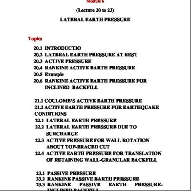
Nptel - Advanced Foundation Engineering-1 4p1m68
December 2019 58
Advanced Engineering Mathematics Lecture Notes 3w3hg
November 2019 100
Advanced Foundation Engineering Question Papers Of Wbut 3t6i30
December 2019 56More Documents from "Sanko Kosan" k1g4s
Advanced Engineering Mathematics Lecture Notes 3w3hg
November 2019 100
Advanced Foundation Engineering Jntuh Notes 6n6x70
April 2020 34
211239040-robert-m-koerner-deg-with-geosynthetics-5-bookfi-org.pdf 2m191v
August 2021 0
Marionette 2566z
December 2019 29